Self calibration

Data required

For this section, you want to continue from your imaging tutorial folder, and you should have the following files.

1. 1252+5634.ms - measurement set containing just the 3C277.1 visibilities.
2. 3C277.1_imaging_outline2026.py - imaging script.
3. 3C277.1_imaging_all2026.py - cheat script containing the answers.
4. 1252+5634_1.clean.* - images, models, residuals (etc.) made during the imaging tutorial.

Table of contents

1. Inspect to choose interval for initial phase self-calibration (4-5)
2. Derive phase self-calibration solutions (step 6)
3. Apply first phase solutions and image again (7)
4. Phase-self-calibrate again (8)
5. Apply the solutions and re-image (9)
6. Choose solution interval for amplitude self-calibration (10)
7. Amplitude self-cal (11)
8. Apply amplitude and phase solutions and image again (12)
9. Summary

1. Inspect to choose interval for initial phase self-calibration (steps 4-5)

← back to top

In this tutorial, we are going to explore the concept of self-calibration. The premise of self-calibration is simple. Instead of using a compact phase reference source (which we assume to be point-like), i.e., flat in amplitude and zero in phase, we assume that the calibrator is resolved. We then derive solutions assuming a model for the true sky brightness. It is called self-calibration because the source we use is often our target source, which calibrates itself. See the lectures for all the gory details on how this works.

As you may have guessed, we require a model of the true sky brightness distribution to perform self-calibration. We have already done this (maybe without you noticing). When we performed our first tclean imaging run, we set savemodel='modelcolumn'. This meant that our model image (our 'best guess' of the real sky) was Fourier-transformed to create model visibilities (stored in the MODEL column of our measurement set). We shall use this model to compare our visibilities against and correct for residual errors.

Let us inspect our model using plotms, as we did in step 1, to plot the model against $uv$ distance.

• Take a look at step 4. The parameters have already been set, so execute the step. You can try overplotting the data and model columns in the same GUI window interactively, or look at the difference between the data and model columns.

  	plotms(vis=target+'.ms',
  		   xaxis='uvdist',
  		   yaxis='amp',
  		   ydatacolumn='model',
  		   correlation='RR,LL',
  		   avgchannel='16',
  		   coloraxis='spw',
  		   plotfile='',
  		   overwrite=True, showgui=gui)

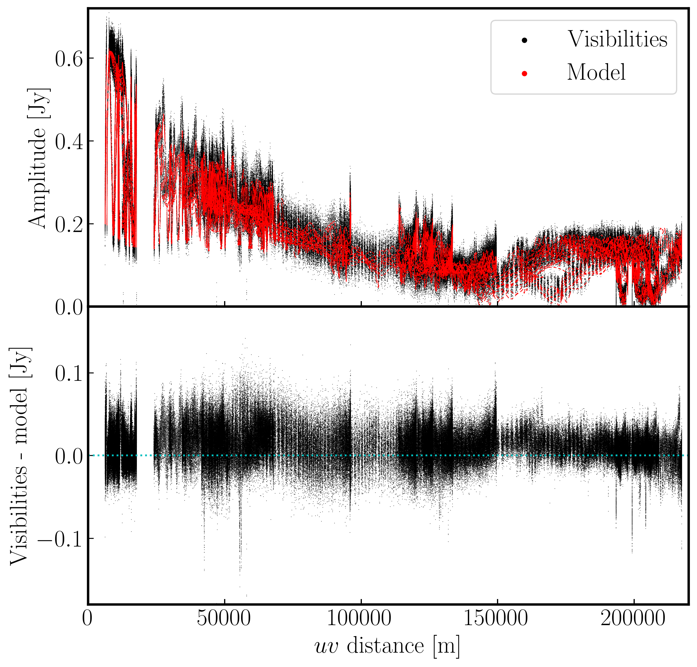
Below, we have overplotted these for convenience in Python. The top panel shows the visibilities (data column) with the model visibilities overlaid. You can see that our imaging-based model is a good approximation to the visibilities. In the bottom panel, the scalar differences are shown, illustrating that the model slightly underestimates the source's flux density across a large $uv$ distance. These discrepancies are due to antenna amplitude errors and will be corrected by self-calibration.

Now that we have our model present, we will begin with phase self-calibration. As with standard calibration, we need to decide what sort of solution interval we require. However, we have an extra complication, namely the source structure.

It can be hard to distinguish phase errors from source structure in the visibilities, but it helps to balance choosing a longer interval to optimise S/N against making it too long (ideally, the phase changes by less than a few tens of degrees). The phase will change most slowly due to source structure on the shortest baseline, Mk2 to Pi, but you should also check the longest baselines (to Cm) to ensure there is enough S/N.

• Take a look at step 5. We want to plot phase against time, averaging across all channels per spw (see listobs for the number of channels).

  	plotms(vis=target+'.ms',
  		   xaxis='**',
  		   yaxis='**',
  		   antenna='**',
  		   correlation='**,**',
  		   avgchannel='**',
  		   coloraxis='spw',
  		   plotfile='',
  		   timerange='',
  		   overwrite=True, showgui=gui)

• Once you are happy, execute step 5 and check the GUI.

  The plot below shows a zoom on a few scans. The chosen solution interval should ideally fit an integer number of times into each scan. It is also advisable not to use too short a solution interval for the first model. This is because the model may not be very accurate, so you don't want to constrain the solutions too tightly.

  

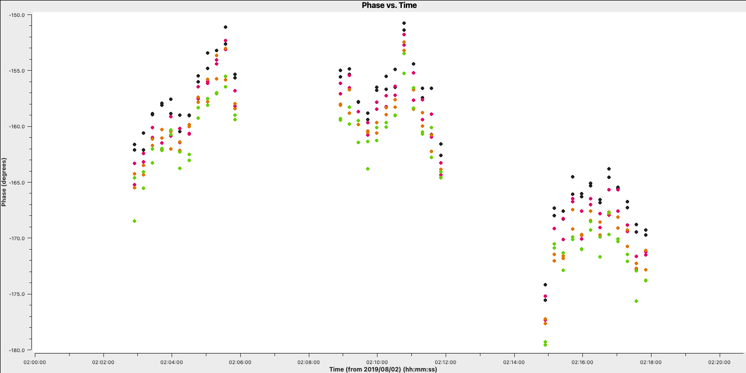
  Looking at this plot, we can see that a 2-4 min solution interval should be sufficient to track the phases without too many failed solutions. Keep your solution interval to hand, as we now want to derive these corrections.

2. Derive phase self-calibration solutions (step 6)

← back to top

Let's use gaincal to compute solutions.

• Take a look at step 6 and enter the parameters in gaincal to perform phase-only calibration with your selected solution interval.

  	gaincal(vis=target+'.ms',
  			calmode='**',          # phase only
  			caltable='target.p1',
  			field=target,
  			solint='**',           # about half a scan duration
  			refant=antref,
  			minblperant=3, minsnr=5)

• We also want to plot these solutions, which are computed separately for both polarisations, using the following code.

  	plotms(vis='target.p1',
  		   gridcols=2, gridrows=3,
  		   xaxis='time', yaxis='phase',
  		   iteraxis='antenna',
  		   coloraxis='spw',
  		   plotrange=[-1,-1,-180,180],
  		   correlation='L',
  		   plotfile='target.p1_L.png', overwrite=True, showgui=gui)
  	os.system('mv Step_06_target.p1_L_*png Step_06_target.p1_L.png')
  
  	plotms(vis='target.p1',
  		   gridcols=2, gridrows=3,
  		   xaxis='time', yaxis='phase',
  		   iteraxis='antenna',
  		   coloraxis='spw',
  		   plotrange=[-1,-1,-180,180],
  		   correlation='R',
  		   plotfile='target.p1_R.png', overwrite=True, showgui=gui)
  	os.system('mv Step_06_target.p1_R_*png Step_06_target.p1_R.png')

• If you are happy, execute step 6
• Check the terminal and the logger; there should be no (or almost no) failed solutions.

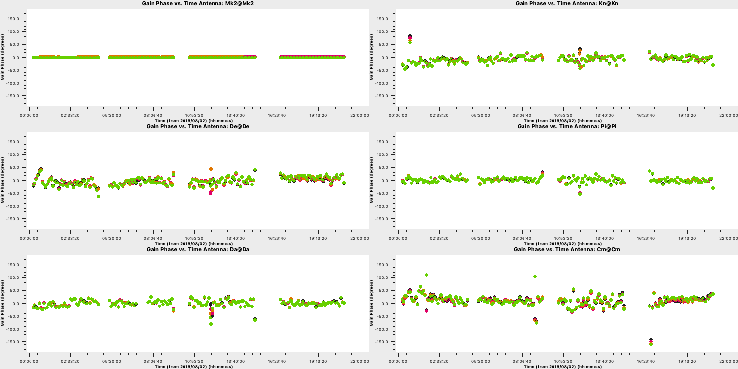
You should have a solution that looks like those below (we used a 180s solution interval). The corrections should be coherent, as they are, and represent the difference caused by the different atmospheric paths between the target and phase-ref, but they may also have a spurious component if the model was imperfect. The target is bright enough that a shorter solution interval could be used. So, these solutions are applied, the data are re-imaged, and the corrections are refined iteratively.

3. Apply first phase solutions and image again (step 7)

← back to top

Let's continue by applying these solutions to the measurement set. Remember that the premise of self-calibration is that we use an iterative approach to gradually improve the calibration of these data. This means we have to obtain a new, improved model (therefore we need to correct these data for imaging).

• Take a look at step 7. There's a lot to enter here, but most of it you have worked out in previous steps. Firstly, we want to enter the calibration table we just made into applycal,

  	applycal(vis=target+'.ms',
  		 	 gaintable=['**']) # enter the name of the gaintable

• Next, we will want to image these data again to generate our new, improved model. The weighting and resolution shouldn't change, so we will use the same parameters as before. Note that the number of iterations has increased, as we expect a higher S/N due to phase self-calibration.
  Linux

  	tclean(vis=target+'.ms',
  		   imagename='targetp1',
  		   imsize=['**','**'],
  		   cell='**arcsec',
  		   deconvolver='clark',
  		   specmode='mfs',
  		   niter=3000, 
  		   cycleniter=300,
  		   threshold=0,
  		   savemodel='modelcolumn',
  		   interactive=True)

  Mac OS

  	iclean(vis=target+'.ms',
  		   imagename='targetp1',
  		   imsize=['**','**'],
  		   cell='**arcsec',
  		   deconvolver='clark',
  		   specmode='mfs',
  		   niter=3000,
  		   cycleniter=300,
  		   threshold=0,
  		   savemodel='modelcolumn')
  	ft(vis=target+'.ms',
  	   model='targetp1.model',
  	   usescratch=True)

• Finally, we want to record the rms and peak brightnesses to see whether there's an improvement. As our imaging parameters are the same, you should try to use the same boxes.

  	rmsp1=imstat(imagename='targetp1.image',
  				 box='**,**,**,**')['rms'][0]
  	peakp1=imstat(imagename='targetp1.image',
  				  box='**,**,**,**')['max'][0]

• If you are happy with all these entries, proceed to step 7. This may take a minute, as the $\texttt{CORRECTED}$ data column needs to be generated.

With these corrections applied, we will CLEAN using (L) tclean / (M) iclean, as before, but you will be able to perform more iterations because the noise should be lower.

Once this is complete, we will obtain the peak and rms values. I obtained $S_p \sim 168 \,\mathrm{mJy\,beam^{-1}}$ and $\sigma \sim 0.282\,\mathrm{mJy\,beam^{-1}}$. This represents a massive $\mathrm{S/N}$ increase to $\sim 595$ from $225$ before phase self-calibration.

Important: A key indicator that self-calibration is improving your data is that the S/N should increase with each iteration. Do not rely on measuring the rms/peak individually, as the self-calibration model could artificially reduce all amplitudes (peak and noise) without any S/N improvement!

4. Phase-self-calibrate again (step 8)

← back to top

Now that the model is better, use a shorter solution interval. Heuristics suggest that 30s is usually about the shortest worth using, because the atmosphere is reasonably stable over these baseline lengths at this frequency.

• Take a look at step 8 and enter the parameters for gaincal as before, but now reduce the solution interval to 30 s.

  	gaincal(vis=target+'.ms',
  			calmode='**',
  			caltable='target.p2',
  			field=target,
  			solint='**',
  			refant=antref,
  			gaintable=['**'],
  			interp=['**'],
  			minblperant=3,minsnr=5)

• Have a look at the rest of the step, which will produce plots of the calibration table.
• When you are happy, execute step 8 and take a look at the plots.

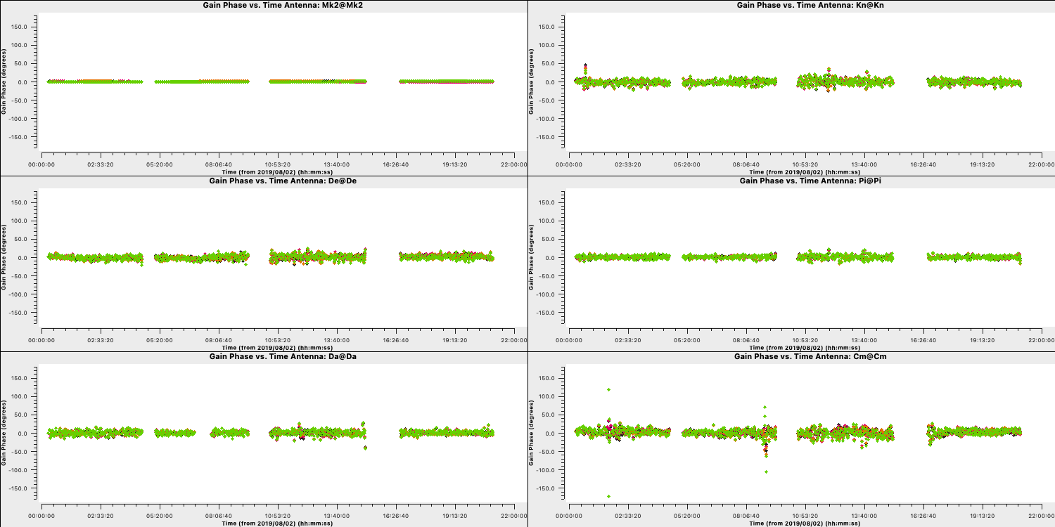
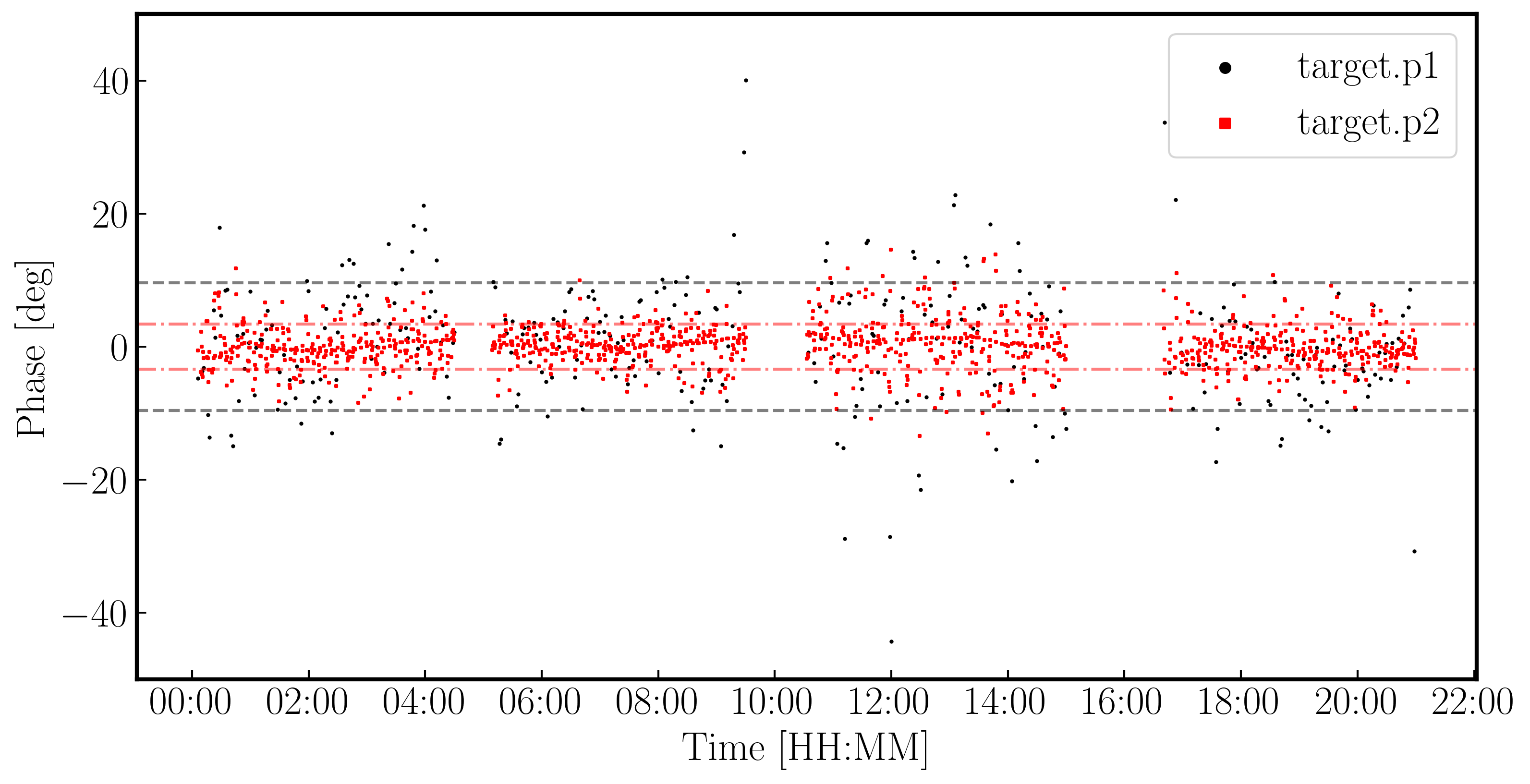
Because we apply the first self-calibration table on the fly, the resulting corrections will be smaller in amplitude than the original corrections. This is a good sign that the self-calibration is working, as the phase errors in your data become smaller. You can see this in the plot below, where we have overplotted the first and second calibration tables, showing that the standard deviation of the solutions decreases (dotted lines). If you find that the solutions are noisier, then something may be going wrong (e.g., too small a solution interval was used).

5. Apply the solutions and re-image (step 9)

← back to top

Let's apply these solutions and reimage.

• Take a look at step 9 and enter the parameters into applycal as before, but make sure we add the new gaintable to the list.

  	applycal(vis='1252+5634.ms',
  			 gaintable=['**', '**'])

We also want to image again in this step. From listobs, the total bandwidth is ~10% of the frequency, which is sufficient for us to need to take the spectral index into account. Cotton et al. (2006) find that the spectral index varies from $-0.1$ in the core to as steep as $-1$.

listobs showed that the total bandwidth is 4817 to 5329 MHz, i.e. for flux density $S$, $S_{4817}/S_{5329} = (4817/5329)^{-1}$, or about 10%. The improved S/N gives much greater accuracy. Thus, to image properly and produce an accurate amplitude image, self-calibration is performed on all spectral windows using multi-term multi-frequency synthesis (deconvolver='mtmfs') imaging. This solves for the sky model that changes across frequency.

• Enter the imaging parameters into the tclean step and the box sizes into the image statistics to track the S/N.
  Linux

  	tclean(vis=target+'.ms',
  		   imagename='targetp2',
  		   imsize=['**','**'],
  		   cell='**arcsec',
  		   specmode='mfs',
  		   niter=4000,
  		   cycleniter=500,
  		   gain=0.2,
  		   threshold=0,
  		   deconvolver='mtmfs',
  		   savemodel='modelcolumn',
  		   nterms=2, # Make spectral index image
  		   interactive=True)

  Mac OS

  	iclean(vis=target+'.ms',
  		   imagename='targetp2',
  		   imsize=['**','**'],
  		   cell='**arcsec',
  		   specmode='mfs',
  		   niter=4000,
  		   cycleniter=500,
  		   gain=0.2,
  		   threshold=0,
  		   deconvolver='mtmfs',
  		   savemodel='modelcolumn',
  		   nterms=2) # Make spectral index image
  	 ft(vis=target+'.ms',
  		model=['targetp2.model.tt0','targetp2.model.tt1'],
  		nterms=2,
  		usescratch=True)

  	rmsp2=imstat(imagename='targetp2.image.tt0',
  				box='**,**,**,**')['rms'][0]
  	peakp2=imstat(imagename='targetp2.image.tt0',
  				box='**,**,**,**')['max'][0]

• Once you are happy, execute step 9 and clean the image! Make sure you clean until as much target flux as possible has been removed into the model - you can increase the number of iterations interactively if you want.
• Use ls to list the names of the image files created. The image is named targetp2.image.tt0.

If we check the image using the same boxes as before, I get $S_p \sim 174.779\,\mathrm{mJy\,beam^{-1}}$ and $\sigma \sim 0.155\,\mathrm{mJy\,beam^{-1}}$. This is another large increase in $\mathrm{S/N}$ to $\sim 1126$.

6. Choose solution interval for amplitude self-calibration (step 10)

← back to top

Now that we have the phases in order, we can work on the amplitudes instead. We first want to determine an appropriate solution interval, so we will use plotms to obtain this information.

• In step 10, use plotms to plot amplitude versus time for the shortest baseline, then execute the step.

  	plotms(vis=target+'.ms',
  		   xaxis='**',
  		   yaxis='**',
  		   ydatacolumn='**',
  		   antenna='**&**',
  		   correlation='RR,LL',
  		   avgchannel='16',
  		   coloraxis='spw',
  		   timerange='',
  		   plotfile='',
  		   overwrite=True, showgui=gui)

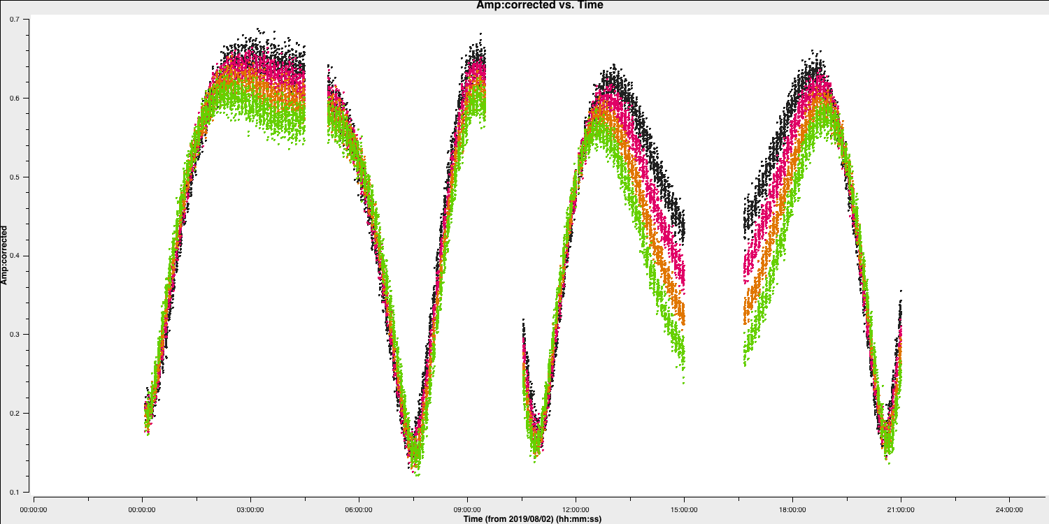
You should find a plot similar to the one below. The smooth amplitude variations throughout the observation are not due to antenna errors but to the source's structure (antenna errors should appear on shorter timescales and be less smooth). Remember that the projected baseline length changes over time, so the sky that the baseline 'sees' also changes.

• To identify a suitable solution interval, we therefore want to zoom in on a few scans using the GUI, as shown below.

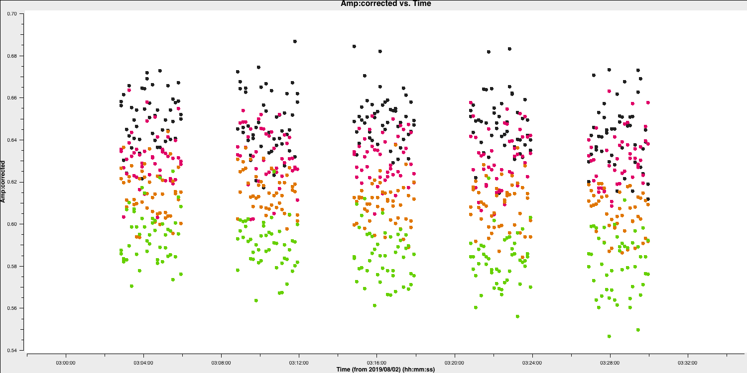
• You can see that, on an integration-to-integration basis, it looks like random noise. Therefore, we want a longer solution interval. Experiment with averaging over different time intervals. A safe starting point would be to combine the solutions per scan (solint='inf').

7. Amplitude self-cal (step 11)

← back to top

In gaincal, the previous gaintable containing short-interval phase solutions will be applied to allow a longer solution (averaging) interval for amplitude self-calibration.

• Take a look at step 11 and set up gaincal to calibrate amplitude and phase, using a longer solution interval and the same refant, etc., as before.

  	gaincal(vis=target+'.ms',
  			calmode='**',
  			caltable='target.ap3',
  			field=target,
  			solint='**',
  			refant=antref,
  			solnorm=True, #Normalise solutions as we have already set the flux scale
  			gaintable=['**','**'],
  			minblperant=3, minsnr=5)

• Once you are happy, execute step 11

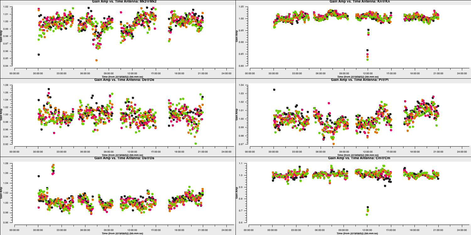
This step will also plot the solutions for each polarisation separately (L polarisation is shown below). They should mostly be within about 20% of unity. A few very low or very high points imply bad data. If the solutions are consistently much greater than unity, the model is missing flux.

8. Apply amplitude and phase solutions and image again (step 12)

← back to top

We are almost finished and now have corrections for phase and amplitude that we can use to remove all these errors. In practice, you may want to run more cycles of self-calibration to further refine the calibration. However, for practical purposes, we are going to apply our solutions and end here.

• In step 12, enter the parameters to apply all calibration tables, generate a final image, and record the statistics for the final image (use the same parameters as before).

  	applycal(vis=target+'.ms',
  			 gaintable=['**','**','**'], calwt=False)

  Linux

  	tclean(vis=target+'.ms',
  		   imagename='targetap3',
  		   imsize=['**','**'],
  		   cell='**arcsec',
  		   specmode='mfs',
  		   niter=5000,
  		   cycleniter=500,
  		   gain=0.2,
  		   threshold=0,
  		   deconvolver='mtmfs',
  		   savemodel='modelcolumn',
  		   nterms=2, # Make spectral index image
  		   interactive=True)

  Mac OS

  	iclean(vis=target+'.ms',
  			   imagename='targetap3',
  			   imsize=['**','**'],
  			   cell='**arcsec',
  			   specmode='mfs',
  			   niter=5000,
  			   cycleniter=500,
  			   gain=0.2,
  			   threshold=0,
  			   deconvolver='mtmfs',
  			   savemodel='modelcolumn',
  			   nterms=2) # Make spectral index image

  	rmsap1=imstat(imagename='targetap3.image.tt0',
  				box='**,**,**,**')['rms'][0]
  	peakap1=imstat(imagename='targetap3.image.tt0',
  				box='**,**,**,**')['max'][0]

• Once you are done, execute the step and clean the image.

For this final image, using the same boxes as before, I obtain $S_p \sim 174.771 \,\mathrm{mJy\,beam^{-1}}$ and $\sigma \sim 87.42\,\mathrm{\mu Jy\,beam^{-1}}$. This is another substantial $\mathrm{S/N}$ increase, from $\sim 1126$ to $1999$.

9. Summary of self-calibration

Although we have completed only three rounds of self-calibration, you should expect to perform additional iterations until the S/N plateaus and no further noticeable improvements are observed in the image. Below, you can see the image improvements at each stage of the self-calibration process and the corresponding improvements in the S/N.

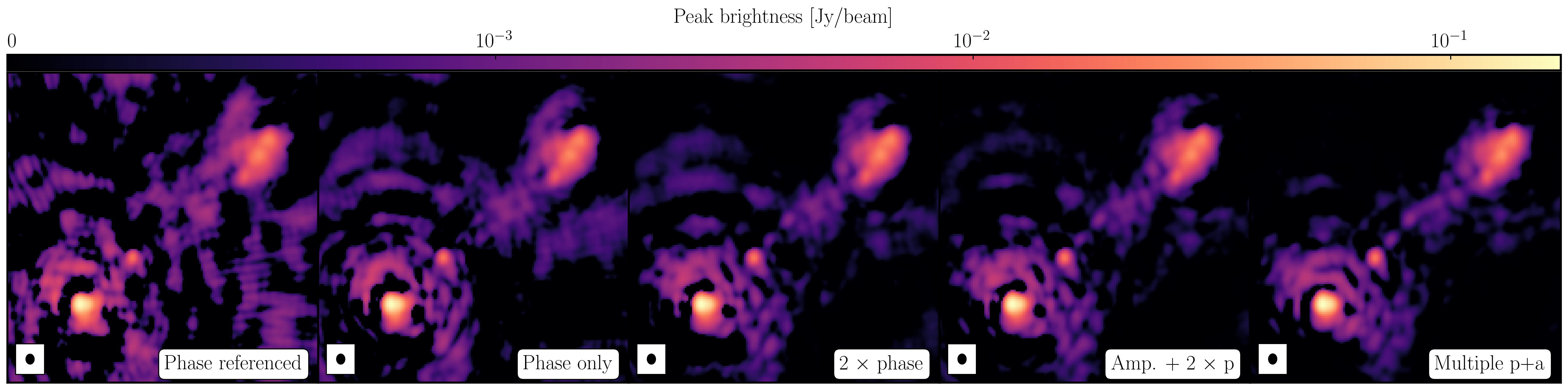
In the rightmost panel, you can see the result if we continue the self-calibration process (reaching 15 and 30 s solution intervals for phase and amplitude, respectively). The majority of these errors have disappeared, image fidelity has improved significantly, and the S/N has peaked at around 3700. Note that not all errors are gone, and specialist algorithms and careful flagging of these data are required to further improve the S/N. For the final tutorial on advanced imaging, we shall use this fully self-calibrated data set.

• Part 5 - advanced imaging