Imaging

Data required

For this section, it is advisable to start with the pre-calibrated data (rather than your own from the calibration section). These are contained in the ERIS26_imaging_tutorial.tar.gz file, which you should already have downloaded. Untar this file and enter the ERIS26_imaging folder that should have been created. Please ensure the following are in your current working directory,

1252+5634.ms - measurement set containing only the 3C277.1 visibilities (this should have been created after the calibration tutorial, or untar the imaging tar bundle (see Home)).
3C277.1_imaging_outline2026.py - imaging script for the next three tutorials (imaging, self-calibration and advanced imaging).
3C277.1_imaging_all2026.py - cheat script containing the answers.

1. Imaging 101

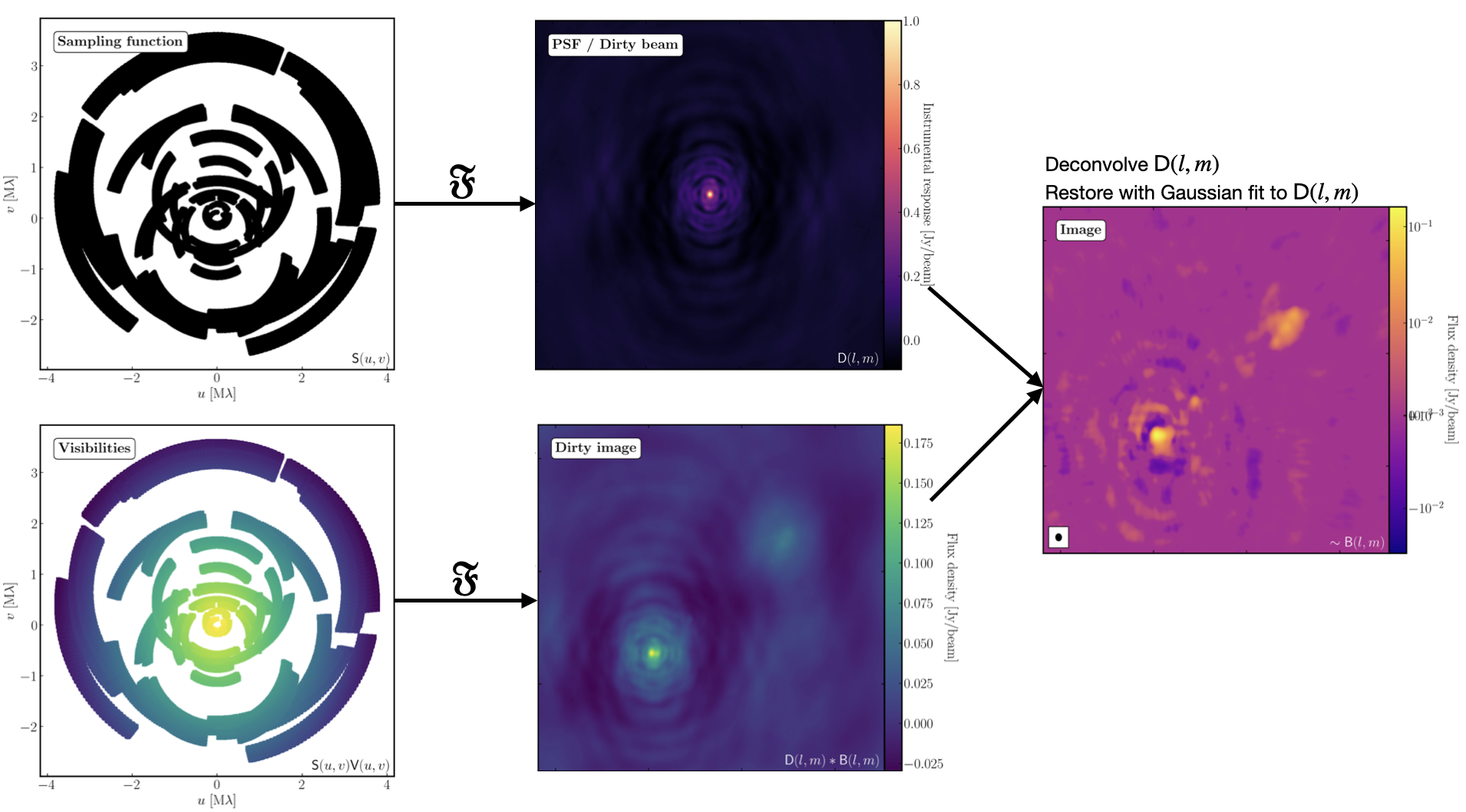
The figure above summarises the imaging process (using our target as an example), and we shall go through it in the following section. As you may recall from the lectures, we can represent the visibilities measured by an interferometer, $\mathsf{V} ( u , v )$, with the following equation: $$\mathsf{V} ( u , v ) \approx \iint _ { l m } \mathsf { B } ( l , m ) \exp\left[ - 2 \pi i ( u l + v m ) \right] \mathrm{d}l \mathrm{d}m$$ where $\mathsf { B } ( l , m )$ is the sky brightness distribution, $l,m$ are directional cosines, and $u,v$ are the coordinates (defined as perpendicular to the source). From the lectures, you will remember that a key factor in interferometric observations is that we have an unfilled $uv$-plane, i.e., we are not sensitive to all spatial frequencies. This makes imaging a fundamentally more difficult problem because we have to deal with arrays with 'holes' in them (also known as sparse arrays). This makes directly Fourier-transforming the visibilities nigh-on impossible.

To address this, we can define a sampling function, $\mathsf{S}(u,v)$, which equals 1 where there is a measurement on the $uv$ plane and 0 otherwise. The sampling function is straightforward to determine because we know exactly where our antennas are at all times, so we know which parts of the $uv$ plane they will occupy. A good way to visualise the $uv$ plane is to imagine the apparent movement of the antennas across the course of the observations, as if you were looking at the Earth from the direction of the source.

If we multiply each side of the imaging equation by the inverse Fourier Transform of the sampling function, we can apply the Fourier Transform ($\mathfrak{F}$) to obtain: $$\mathsf{ B } ( l , m ) * \mathsf{ D } ( l , m ) \approx \iint _ { uv } \mathsf{S} ( u , v ) \mathsf{V}( u , v ) \exp\left[ 2 \pi i ( u l + v m ) \right] \mathrm{d}u\mathrm{d}v \\\mathsf{ D } ( l , m ) = \iint _ { u v } \mathsf{S} ( u , v ) \exp\left[ 2 \pi i ( u l + v m )\right] \mathrm{d}u \mathrm{d}v$$ where $\ast$ is the convolution operator. You can see that we can now recover the intrinsic source brightness distribution $\mathsf{B}(l,m)$ if we can deconvolve the $\mathsf{D}(l,m)$ term from it. This $\mathsf{D}(l,m)$ term is known as the dirty beam or point spread function (PSF). Fortunately, this can be derived easily because we know exactly what $\mathsf{S}(u,v)$ is.

Sounds simple, eh? Not so! The next step, namely deconvolving the PSF from the dirty image, is a little more complicated than it sounds. The deconvolution process is called an 'ill-posed' problem in mathematics. This means that, without some assumptions, solutions to deconvolution are often not unique, i.e. there are many variants of $\mathsf{B}(l,m)$ that would satisfy the equation. In addition, the algorithms used to perform deconvolution can be highly non-linear and can diverge from 'good' solutions.

To help the deconvolution process, we can apply a range of assumptions to guide it towards the most likely sky brightness distribution. These assumptions are often physically based, e.g. the assumption that $\mathsf{B}(l,m)$ is always positive, but they can vary slightly with each deconvolution algorithm.

The most commonly used algorithms are the CLEAN variants, which we shall discuss here. The standard CLEAN algorithm (either Högbom or Clark) assumes that the sky is sparse, i.e., radio sources are far from each other, and that the sky brightness distribution can be represented by point sources (i.e. delta functions). The CLEAN algorithm iterates through many cycles, identifying the brightest pixels, removing 10% (the default value) of the flux density at each of these pixels, and recording the value and position in a model image. CLEAN then calculates the contribution of these removed pixels, convolved with the PSF, and subtracts it from the dirty image. This is known as a 'minor cycle'.

After a certain number of minor cycles, the model is Fourier transformed and subtracted from the visibility data, which are then re-Fourier transformed to produce a new dirty image with less bright emission and fewer contributions from the dirty beam. This is known as a 'major cycle'. These cycles are continued until the final dirty image (or the 'residual image') is indistinguishable from noise. The following plot shows the CLEAN process on 3C277.1, which we are about to image. You can see how the model is built up and how the contribution from the PSF decreases over each major cycle and each CLEAN iteration (which, by default, removes 10% from the brightest pixel).

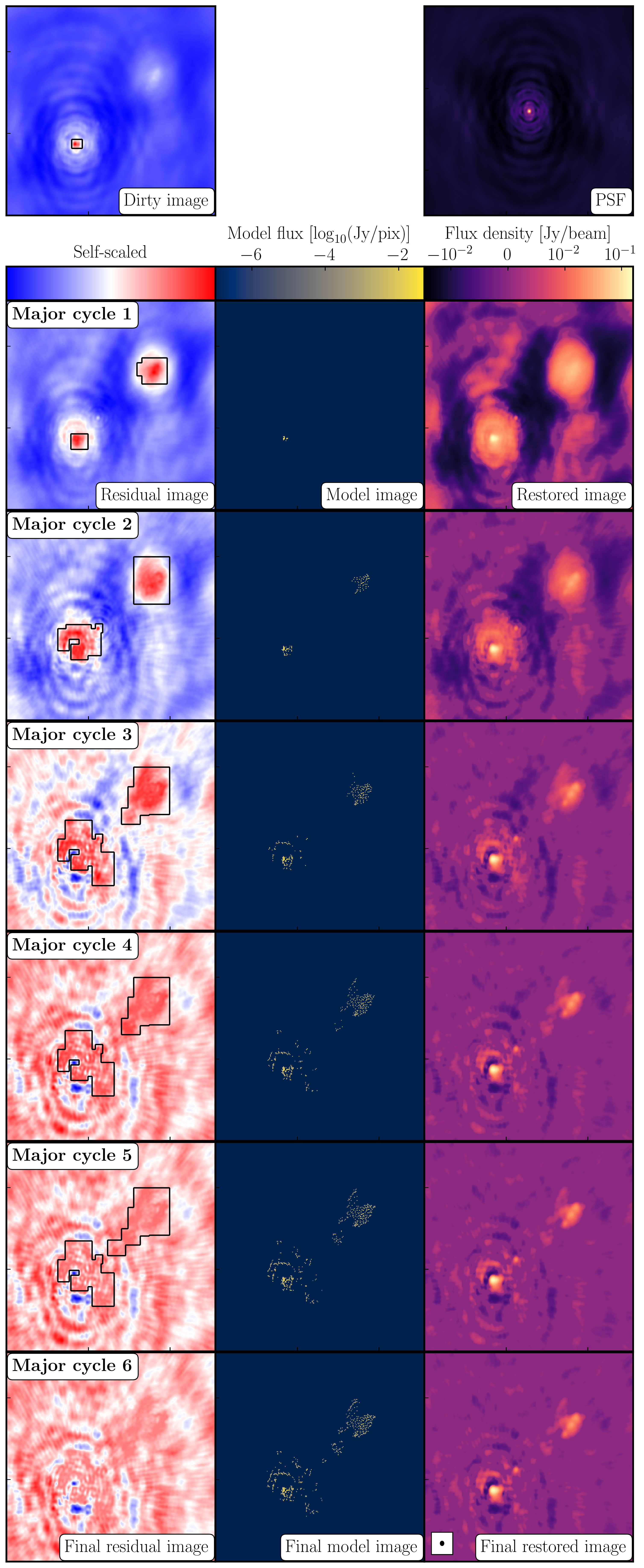
Once deconvolution is complete and the residual image looks close to noise, the model is convolved with the synthesised beam and added back to the data (without the horrible sidelobes). The synthesised or restoring beam is an idealised Gaussian fit to the PSF and can be thought of as the effective resolution of the interferometer array. The final image is shown in the rightmost panel of the figure at the start of this section. The synthesised beam size is represented by the elliptical overlay in the bottom left of the image.

2. Determining the imaging parameters (steps 1-2)

← back to top

Let's get on with making our first image using the CASA task tclean. At the CASA prompt, type default(tclean) and then inp. There are quite a few inputs, which can be daunting. However, this task is very versatile and supports imaging for many different observing set-ups (e.g. spectral line, wide-field, etc.). If you are unsure what is best for your data, consult the CASA docs. Note that for Mac OS users, we will be using a task called iclean. This is functionally the same as tclean and is simply a wrapper that provides the GUI for interactive cleaning, because the casaviewer has been deprecated on Mac OS.

Important: In the following sections, Linux-specific help will start the sentence with a (L) and Mac-specific help with a (M).

Take a look at step 2 and fill in the empty parameters using the information and instructions provided below.

Linux

	tclean(vis=target+'.ms',
		   imagename='target1',
		   specmode='mfs',
		   niter=1500,
		   cycleniter=300,
		   threshold=0,
		   imsize=['**','**'],
		   cell='**',
		   weighting='**',
		   deconvolver='**',
		   savemodel='modelcolumn',
		   interactive=True)

Mac OS

	iclean(vis=target+'.ms',
		   imagename='target1',
		   specmode='mfs',
		   niter=1500,
		   cycleniter=300,
		   threshold=0,
		   imsize=['**','**'],
		   cell='**',
		   weighting='**',
		   deconvolver='**',
		   savemodel='modelcolumn')
	ft(vis=target+'.ms', 
	   model='target1.model',
	   usescratch=True)

There are some things that we always need to decide and set when imaging, which are:

imagename - this is self-explanatory. You need to set an image name that should describe the imaging step and the object imaged.
field - this is the name of the field/source you want to observe, and it is self-explanatory.
cell is the angular size of each pixel in our output image. To estimate this, we need to determine the resolution of our interferometer. We can do this by examining the $uv$ distance (i.e. the radial distance of measurements in the $uv$ plane). This is done in step 1 of your 3C277.1_imaging_outline2026.py script.
- Either execute step 1 or use the following commands.
```
	plotms(vis='1252+5634.ms',
		   xaxis='uvwave',
		   yaxis='amp',
		   correlation='RR',
		   avgchannel='16',
		   spw='3',
		   showmajorgrid=True,
		   showminorgrid=True,
		   plotfile='',
		   overwrite=True)
```
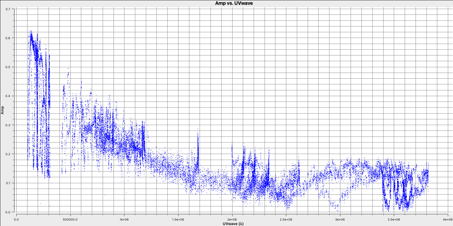
Only the highest-frequency spectral window is chosen (as this corresponds to the best resolution, remember $\lambda/B$), and only one correlation is selected. These choices are made to improve the plotting time.
In this plot, the greatest projected baseline length of the observation corresponds to the highest possible resolution of your observation. Note that we have plotted this in units of wavelength to simplify the calculation.

To obtain a good value for the cell size, you should read the highest $uv$ distance value (which is approximately $3.8\times10^{6}\,\lambda$). With this value in hand, we can convert it into a representative resolution (remember the resolution of an interferometer is $\sim\lambda/D$ and the $\lambda$s will cancel out!).

There is one other factor we have missed, namely Nyquist sampling ($N_\mathrm{s}$). Remember that, during imaging, we have to fit a 2D Gaussian to the PSF to obtain our synthesised/restoring beam. The minimum number of pixels required to fit a Gaussian is at least 3, but often (especially for sparse arrays where the PSFs are highly non-Gaussian) more pixels are used.

Based on the aforementioned points, an estimate for a suitable cell size is given by the following equation: $$\mathrm{cell} \approx \frac{180}{\pi N_\mathrm{s}} \times \frac{1}{D_\mathrm{max}\,\mathrm{[\lambda]}}~\mathrm{[deg]}$$ In this case, assuming $D_\mathrm{max} = 3.8\times10^{6}\,\lambda$ and $N_\mathrm{s} = 4$ pixels, you should obtain a cell size of around $13.5\,\mathrm{milliarcseconds~(mas)}$, i.e. cell=['13.5mas'].
imsize - This sets the number of pixels along each side of the image. It is often a compromise between computing speed and deconvolution performance. You want an image that is not too large, but large enough to remove the PSF sidelobes (see the imaging figure above!). If your source is extended, the image size may also need to be larger to account for this. In addition, we want to set an image size that is optimal for the underlying algorithms in tclean. According to CASA, a good choice is an even number that is divisible only by 2, 3, 5 and 7, or a factor of $2^n$!. An easy rule of thumb is to use an image size of $2^{n}\times 10$, where $n$ is an integer.

Our source is extended, so we want an image large enough to cover all the emission. To find a suitable image size, see Ludke et al. 1998 page 5 and estimate the size of that image in pixels. You should find that an image size of about 256 should be sufficient, i.e., imsize=[256,256]
deconvolver - The choice of deconvolution algorithm depends on your source and your interferometer. To establish the correct choice for your data, consult the CASA docs. A good rule of thumb for what to pick is the following:
- Do you expect your sources to be extended, i.e. $\gg$ the resolution? Consider multiscale (this deconvolution algorithm assumes the sky comprises many Gaussians, which is better for modelling fluffy emission than using delta functions)
- Does your observation have a large fractional bandwidth, i.e., a good rule of thumb is $\mathrm{total~bandwidth/central~frequency} = \mathrm{BW}/\nu_c > 15\%$? Consider mtmfs (this models changes in the source's flux/morphology across the bandwidth, and failing to model this can cause un-deconvolvable errors in the image)
  If the source is also extended, implement multiscale deconvolution by setting the scales parameter.
- Do you expect the source to have polarisation structure? - consider clarkstokes (which cleans the polarisations separately)
- If not, we would expect to have a small bandwidth and a compact structure, so the clark algorithm should be sufficient.
In our case, we have a borderline fractional bandwidth ($\mathrm{BW}/\nu_c \sim 0.512\,\mathrm{GHz}/5.072\,\mathrm{GHz} \sim \mathbf{10\%}$), and we don't care about polarisation. This means that setting deconvolver='clark' should be fine (note that we will try multiscale in the advanced imaging tutorial).
niter - following on from the deconvolver, this parameter determines the number of iterations the deconvolution algorithm will use. As mentioned earlier, at each iteration a percentage of the flux of the brightest pixel is removed from the dirty image; therefore, the larger the niter, the more flux is removed. Luckily, we are going to do this interactively and inspect the residuals after each major cycle, so we can adjust niter on the fly. For this, we won't go so deep, so we set niter=1500. (L) We will do it interactively, so set interactive=True. (M) For Mac users, we shall use iclean to do interactive cleaning. Note that if we didn't do it interactively, you could use tclean on Mac OS.
weighting - the weighting parameter determines how the various baselines are represented in the imaging routine. Uniform weighting gives each baseline in the $uv$ plane equal weight, which typically yields the highest resolution, whilst natural weighting maximises sensitivity and increases the contributions from data points/baselines that are closer in the $uv$ plane. For this imaging, we shall use the default weighting='natural'. We shall investigate the effects of changing the weighting in the advanced imaging section.

3. First image of 3C277.1 (step 2)

← back to top

With the imaging parameters set in step 2, we want to start imaging our source.

Execute step 2 and check the logger. The algorithm will grid the visibilities with the appropriate weights and produce the PSF, ready for deconvolution and for inverting the visibilities to produce our dirty image. We can guide the deconvolution process to prevent divergence (as explained in part 9).
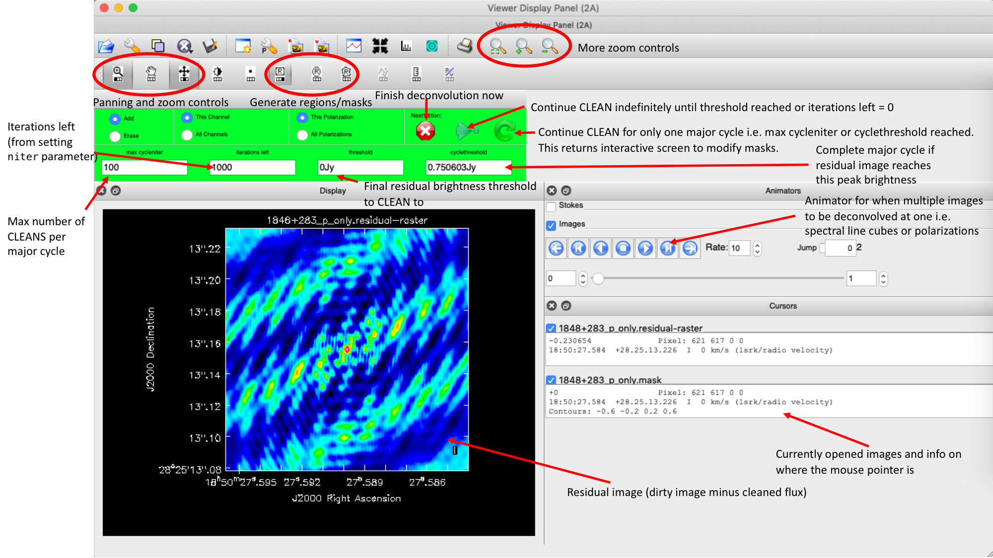
The guidance comes via masks. These masks tell the algorithm which pixels to search for flux to be removed and for PSF deconvolution. These masks should be set in regions that you think contain real flux. They typically match the PSF shape for point sources (see part 9 of this section for the PSF shape). Because we set (L)interactive=True / (M) used iclean, CASA returns a GUI similar to that shown below, where we can set masks and guide the deconvolution process.

Linux

Mac OS

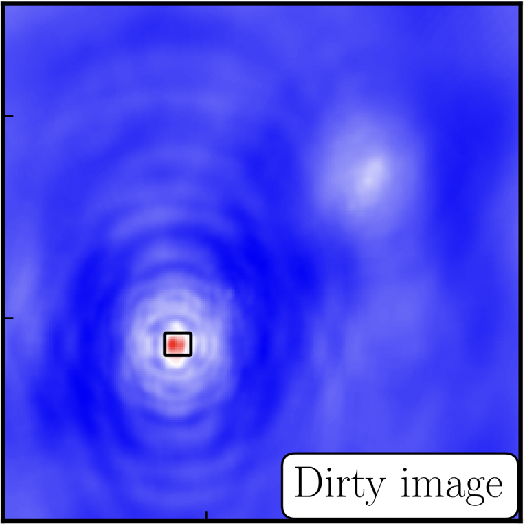The GUI will display the dirty image. At the bottom left of the image, there is a bright source with the characteristic PSF shape around it. This is where we want to begin setting our mask. The figure to the right shows the dirty image, with the black contour indicating an example of a good first mask.
To set the mask, we want to use the region buttons (e.g. (L) / (M) ). (L) The filled rectangle among the three on these buttons corresponds to the mouse buttons. (L) These can be adjusted and reassigned to different mouse buttons by clicking on them.
The gif below shows how to set the mask and run the next major cycle. Important note that to set the mask, we need to (L) double-click with the appropriate button (in this case, the right mouse button) or (M) press shift+a. The box should change to a solid line. Set a mask around the brightest regions and clean interactively, masking new regions or increasing the mask size as needed. A guide to setting a mask is shown in the gif below.

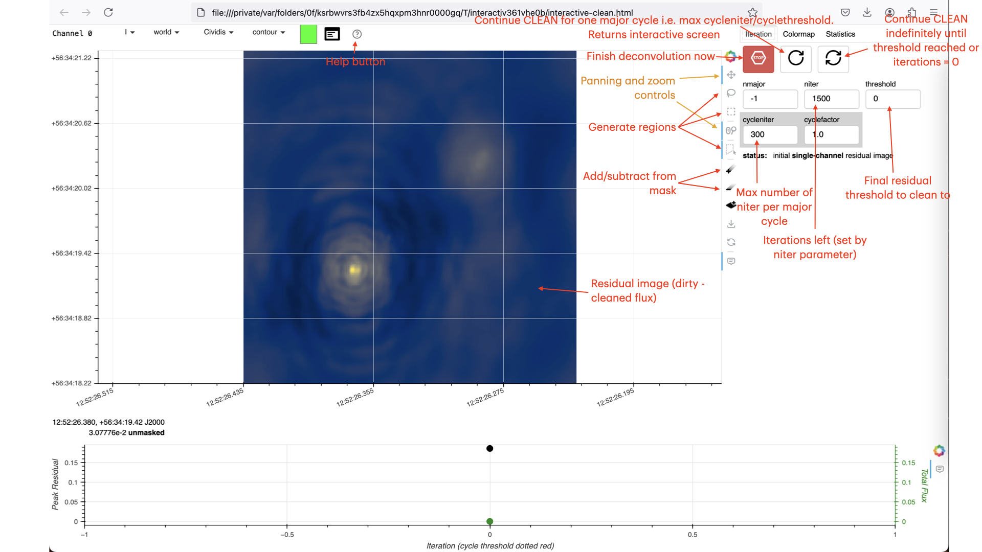
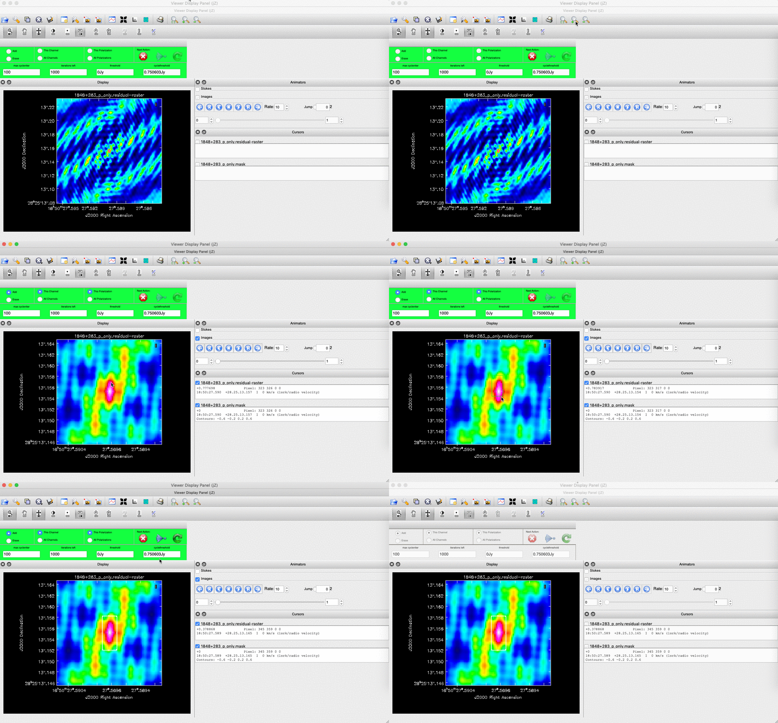
Once the green arrow (L) or single circular arrow (M) button is pressed, the next major cycle will run and the GUI will freeze. This process will remove some flux, deconvolve the PSF, and begin generating the model, as explained in part A. Once these contributions have been removed from the visibilities, the task will generate another residual image with less bright flux and re-open the imview GUI.
Continue with the cleaning process and modify the mask as appropriate. You can delete parts of the mask by clicking the erase button, placing the green box over the region to remove, and double-clicking to remove that portion.
Over the course of the CLEAN process, you should see the PSF imprint being removed and the residual turning into noise (or noise plus calibration errors). The plot from earlier, showing the deconvolution process illustrates this.
After about 2 major cycles, you should see some low-flux-density structure appear, which we then need to CLEAN. This is why we modify our mask, as this was unseen in the dirty image.
Continue until around major cycle 6, when the source becomes indistinguishable from noise, then click the red cross to stop cleaning.

With CLEAN stopped and completed, the algorithm shall take the model image (the delta functions), convolve it with the fitted PSF (i.e. the synthesised beam), and add this to the residual image to generate the image. Let's have a look at what CLEAN has made.

Type !ls into the CASA prompt.

You should see some new files, which are CASA images. These are:

target0.image - The model, convolved with the synthesised beam, is then added to the residual image.
target0.residual - The noise image after CLEAN deconvolution (seen in the interactive prompt during CLEANing).
target0.model - The underlying estimated sky brightness model by CLEAN.
target0.psf - The FT of the sampling function used for deconvolution.
target0.pb - The primary beam response across the image (Note this is not correct for heterogeneous arrays).
target0.sumwt - The sum of weights (not needed).

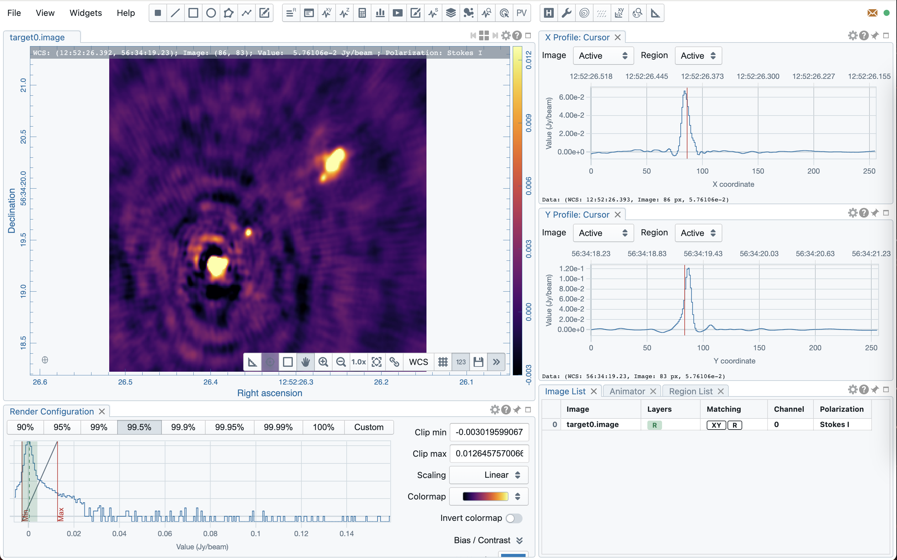
(L) Type imview at the CASA prompt / (M) open CARTA to view these images. Try to determine where these images originate by comparing them with the imaging 101 section.
Look at the target0.image. The source shows some structure, but the background noise appears non-Gaussian, with stripes and negatives in a non-random pattern. This is a tell-tale sign of calibration errors. We shall address these errors in the self-calibration section.

4. Measuring image properties (step 3)

← back to top

Now that we have produced the first image, we want to extract some properties from it. You will need to do this to extract your science, and in this case we are going to do it to track the calibration improvements in the next tutorial (on self-calibration).

Take another look at your image using (L) imview or (M) CARTA. The synthesised beam is displayed and measures about $64\times53\,\mathrm{mas}$ for this image.
To track calibration improvements, we want to measure the root-mean-square (rms) noise level ($\sigma$) and the peak brightness ($S_\mathrm{p}$) so that we can calculate the signal-to-noise ($\mathrm{S/N} = S_\mathrm{p}/\sigma$). To do this, we can use the set a region tool. We want a region with no source flux so we can measure the rms noise (see the statistics tab), and another region over the brightest emission to measure the peak brightness. Try this interactively first, and record your values for the peak, rms noise and S/N.
To automate this process, we can also use the task imstat and select the boxes via the inputs. See step 3 and enter the box values (note that the box format is box = "x_bottom_left_corner, y_blc, x_top_right_corner, y_trc")
```
	rms1=imstat(imagename='target0.image',
				box='**,**,**,**')['rms'][0]
	peak1=imstat(imagename='target0.image',
				box='**,**,**,**')['max'][0]

	print(('target0.image rms = %7.3f mJy' % (rms1*1000.)))
	print(('target0.image peak = %7.3f mJy/bm' % (peak1*1000.)))
	print(('target0.image S/N = %7.3f' % (peak1/rms1)))
```
(L) The other command in step 3 demonstrates how to use imview to produce reproducible images. This is optional but included for reference. You can use imview interactively to determine parameter values. Note: If you use it interactively, ensure the black area is just large enough to enclose the image; otherwise, imview will produce a strange aspect ratio plot. (M) On Macs, you can save the image in CARTA as a PNG.
```
		imview(raster={'file': 'target0.image',
					   'colormap':'Rainbow 2',
					   'scaling': -2,
					   'range': [-1.*rms1, 100.*rms1],
					   'colorwedge': True},
			   zoom=1,
			out='target0.image.png')
```
- Execute step 3, and you should see the rms and peak brightness displayed on the screen. Calculate the S/N and record these values for later. You should also have a saved plot like the one shown below.
I managed to achieve a peak brightness of $S_\mathrm{p} = 160.96\,\mathrm{mJy\,beam^{-1}}$ and an rms noise level of $\sigma = 0.71\,\mathrm{mJy\,beam^{-1}}$, corresponding to an $\mathrm{S/N} \approx 225$. You should find values similar to these ($\mathrm{S/N} \sim 160\mbox{--}240$). If you did not, check your residuals to ensure you cleaned deeply enough, or retrace your calibration steps.
Linux / imview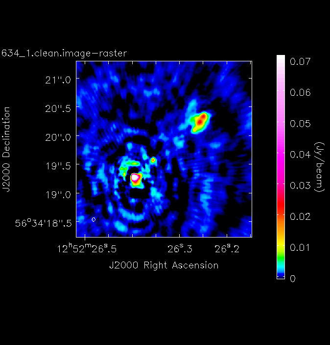 Mac OS / CARTA
Congratulations, you have finished the imaging part of this tutorial. Next, we shall move on to removing these final calibration errors using this image. Follow the link below to continue.
- Part 4 - self-calibration

Imaging

Data required

Table of contents

1. Imaging 101

2. Determining the imaging parameters (steps 1-2)

3. First image of 3C277.1 (step 2)

4. Measuring image properties (step 3)