Calibration
Data required
This tutorial continues with the same dataset and set of Python scripts as the first tutorial. You should have at least the files in your current working directory,
all_avg.ms- the data (after conversion to a measurement set).3C286_C.clean.model.tt0- used for fluxscaling of the data set.all_avg_all.flags.txt- all flags0319+4130_flags.txt- empty flagging file for bandpass calibrator0319+4130_flags_answers.txt- complete flagging file for bandpass calibrator3C277.1_cal_outline2026.py- the script that we shall input values into to calibrate these data.3C277.1_cal_all2026.py- cheat script for calibating these data.
Important: Before you begin this tutorial, we want to ensure that your data sets are identical (to save time). Please enter the following two commands at a CASA prompt to ensure the flagging is identical:
runsteps=[10]
execfile('3C277.1_cal_outline2026.py')
Table of contents
- Setting the flux of the primary flux scale calibrator (11)
- Bandpass calibration
- Decorrelation and solution intervals (12)
- Pre-bandpass calibration (13)
- Derive bandpass solutions (14)
- Time-dependent delay calibration (15)
- Gain calibration (17)
- Time-dependent phase calibration of all calibration sources
- Time-dependent amplitude calibration of all calibration sources
- Determining true flux densities of other calibration sources (18-19)
- Apply solutions to target (20-21)
1. Setting the flux of the primary flux scale calibrator (step 11)
The first step is to set the flux density of the flux scale calibrators (in this case, 3C286 and 3C84). This is important because the correlator outputs the visibilities with an arbitrary scaling, so they are not in physical units, i.e., Janskys. However, the visibility amplitudes are correct relative to each other. This means that we can observe a standard source with a physically known flux density (similar to the zero points of a temperature scale), which can then be used to rescale the visibilities and put all fields onto this scale.
In this observation, we found that 1331+3030 (= 3C286) is an almost non-variable radio galaxy, and its total flux density is very well known as a function of time and frequency (Perley & Butler 2013). However, this flux density standard was derived from VLA observations, and the source is somewhat resolved by e-MERLIN.
To mitigate this, we use a model derived from a ~12 hr observation centred on 5.5 GHz. This is scaled to the current observing frequency range (around 5 GHz) using setjy, which derives the appropriate total flux density, spectral index and curvature from parameters in Perley & Butler (2013).
However, a few per cent of the flux is resolved out by e-MERLIN; the simplest way (at present) to account for this is to scale the fluxes derived for the other calibration sources by 0.938 (based on calculations for e-MERLIN by Fenech et al.).
The model consists of delta functions, and setjy enters them into the Measurement Set so that their Fourier Transform can be used as a $uv$-plane model for later comparison with the actual visibility amplitudes. If you make a mistake (e.g. setting a model for the wrong source), use the task delmod to remove it.
- Take a look at step 11. Enter the correct parameters for the
setjytask and for the flux scaling of 3C286.setjy(vis='**', field='**', reffreq='5.073e9Hz', standard='Perley-Butler 2013', spix=-0.66, model='**', usescratch=True) # You should have downloaded and decompressed this model - Have a look at the other commands in step 11, which are completed for you. By default,
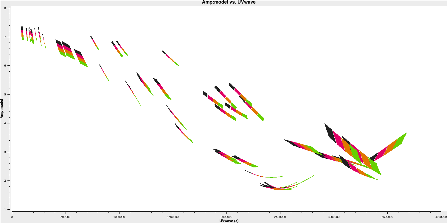
setjyscales the model for each channel, as seen when you plot the model amplitudes against $uv$ distance, coloured by spectral window. The firstplotmscommand (shown below) plots the model against $uv$ distance. The model appears only for the baselines present during the short time interval for which 1331+3030 was observed here.plotms(vis='all_avg.ms', field='1331+3030', xaxis='uvwave', yaxis='amp', coloraxis='spw',ydatacolumn='model', correlation='LL,RR',symbolsize=4, showgui=gui,overwrite=True, plotfile='3C286_model.png')
- While this is not standard for e-MERLIN data, we are also setting the flux density of the bandpass calibrator (0319+4130) in this step. Normally, we would derive its flux density from 3C286 and then perform the bandpass calibration twice (once without accounting for spectral indices and once with). This source is well known, so, to avoid extra calibration steps, we are going to set its flux density here and the spectral index,
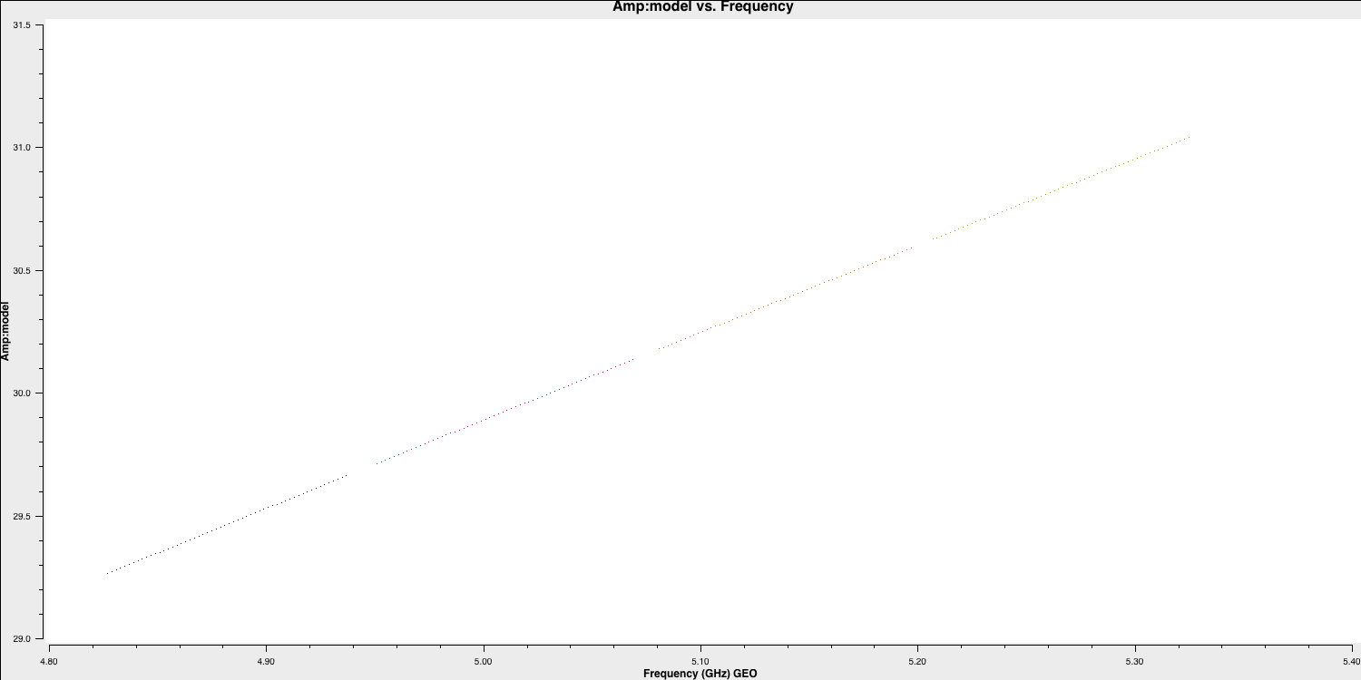
spix, with the following code (done for you).setjy(vis='all_avg.ms', field='0319+4130', standard='manual', fluxdensity=[30.1388, 0.0, 0.0, 0.0], spix = 0.6, reffreq= '5.07GHz') - This source is not resolved by e-MERLIN; therefore, the model we will use is a point source. Hence, the following
plotmsstep should show a slope of 0.6 in amplitude versus frequency, with a flux density of $30.1388\,\mathrm{Jy}$ at $5.07\,\mathrm{GHz}$.plotms(vis='all_avg.ms', field='0319+4130', xaxis='freq', yaxis='amp', coloraxis='spw',ydatacolumn='model', correlation='LL,RR',symbolsize=4, showgui=gui,overwrite=True, plotfile='3C84_model.png')
2. Bandpass calibration
2A. Investigating decorrelation and solution intervals (step 12)
We have set the primary fluxes of the main flux/bandpass calibrators, and we can now move on to calibrating for instrumental and atmospheric effects. If you remember from your introduction to interferometry, we used a model of the locations of our telescopes to correct for the geometric delay and ensure that our signal from the source interferes constructively across all antennae. However, the atmosphere, electronics and engineering of the antennae, and clock and timing errors change the phase and prevent perfect constructive interference. We therefore have to correct for this.
To correct for this, our standard calibration assumes that your calibrator sources are point-like (i.e., flat in amplitude and zero in phase). This means that any deviation must be due to an error. Secondly, there is an assumption that the errors are antenna-independent, i.e., there must be a common factor/error on each baseline to the same antenna. This is sensible, as each antenna will have different clocks (in the case of VLBI), different atmospheric line-of-sights, different LNAs, etc. This also means that we should be able to derive a per-antenna solution and prevents us from simply making our visibilities look like a point source (if we solved per baseline).
We are going to calibrate the bandpass calibrator (0319+4130) first, with the goal of generating a bandpass calibration table. The bandpass is the antenna's response (amplitude and phase) as a function of frequency. This varies rapidly with frequency but is not expected to change with time (at least during the observation), as it is typically due to filters and receiver sensitivities within the antenna. This means we need to obtain solutions for each channel, so we need a very bright source (0319+4130 is 20-30 Jy, so very bright) to provide sufficient signal in each small channel bandwidth. However, before we can derive this correction, we need to first calibrate the other sources of error affecting this source, in order to isolate the bandpass correction.
To begin, we will correct for the phase errors, $\Delta\phi$, which can be parameterised primarily by a constant plus higher-order terms: $$\Delta\phi = \phi_{0}(t,\nu) + \frac{\partial \phi}{\partial \nu}\Delta\nu + \frac{\partial \phi}{\partial t}\Delta t$$ We call $\phi_0(t,\nu)$ the phase error, $\frac{\partial \phi}{\partial \nu}\Delta\nu$, the slope in frequency space, the delay error, and $\frac{\partial \phi}{\partial t}\Delta t$, the slope against time, the rate error. The rate error and higher-order terms are typically needed only for long baselines or low frequencies, where more turbulent atmospheric conditions and separate clocks cause errors. Most modern interferometers, including e-MERLIN, often need to consider only the delay and phase terms.
- Take a look at step 12. It is advisable to copy the individual
plotmscommands directly into CASA for this step. - Copy the first command into CASA to plot the phase versus time for a bright source, i.e., our bandpass calibrator (so we can see the visibilities above the noise). Note that we are selecting only one scan of this source.
	plotms(vis='all_avg.ms', field='0319+4130',
	       xaxis='frequency',yaxis='phase',
	       gridrows=5,gridcols=1,iteraxis='baseline',
	       xselfscale=True,xsharedaxis=True,
	       ydatacolumn='data',antenna=antref+'&*',
	       avgtime='2400',correlation='LL,RR',
	       coloraxis='corr', scan='92',
	       plotfile='',plotrange=[-1,-1,-180,180],
	       showgui=gui,                    # change to True to inspect by interval or antenna
	       overwrite=True)
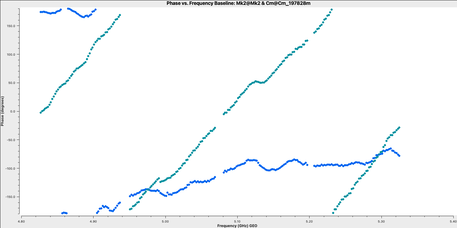
The $y$-axis spans $-180$ to $+180$ deg, and some data show a slope of about a full 360 deg across the 512 MHz bandwidth. Looking at the baseline to the Cambridge telescope, think about the following questions.
QUESTION 1: What is the apparent delay error that this corresponds to? What will be the effect on the amplitudes?
QUESTION 2: Delay corrections are calculated relative to a reference antenna, which is assumed to have zero phase, so the corrections factorised per other antenna include any correction due to the reference antenna. Roughly, what do you expect the magnitude of the Cambridge telescope corrections to be? Do you expect the two polarisation hands to have the same sign?
- Have a look at the second and third
plotmscommands, which show what happens if we average these data without correcting for the delay slope. The first command plots the amplitude of one channel and one correlation on the longest baseline.
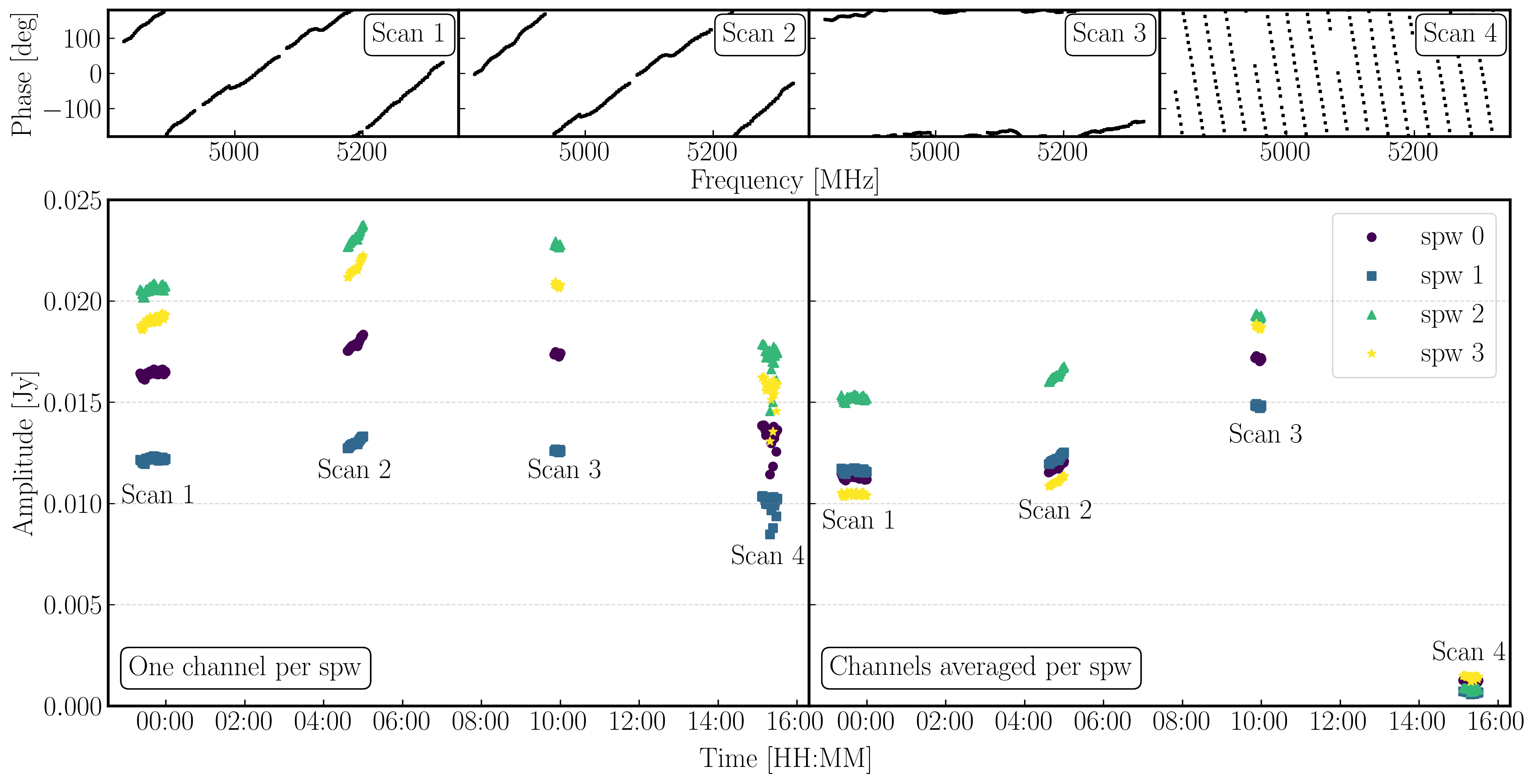
The next command plots the same but now we are averaging the channels together,plotms(vis='all_avg.ms', field='0319+4130', spw='0~3:55', ydatacolumn='data', # Just one channel per spw yaxis='amp', xaxis='time', plotrange=[-1,-1,0,0.025], # Plot amplitude v. time with fixed y scale avgtime='60',correlation='RR', antenna=antref+'&Cm', # 60-sec average, one baseline/pol coloraxis='spw',plotfile='', showgui=gui, overwrite=True)plotms(vis='all_avg.ms', field='0319+4130', xaxis='time', yaxis='amp',ydatacolumn='data', spw='0~3',avgchannel='64', antenna=antref+'&Cm', avgtime='60',correlation='RR', plotrange=[-1,-1,0,0.025],coloraxis='spw', plotfile='', showgui=gui, # change to T to inspect closely overwrite=True) - QUESTION 3: Take a look at the two plots and compare them. Which has the higher amplitudes - the channel-averaged data or the single channel? Why?Click for answerThe single channel has higher amplitudes. The source 3C84 is very bright, so there is plenty of signal in each single channel. However, averaging over all channels when there is a large phase slope causes the amplitudes to decorrelate, so the channel-averaged data have depressed amplitudes. A similar effect is seen if you have data with phase errors as a function of time and average over too long a time period.
We have plotted the amplitude versus time plots below in Python for the four scans of the bandpass calibrator. As you can see, the effects of decorrelation of the amplitudes are more pronounced when the delay error is larger (e.g., in scan 4).
Finally, in preparation for the calibration of the bandpass source, we want to derive the time-dependent phase solution interval. A solution interval is simply the amount of time you average together to derive a correction. Selecting a solution interval can be tricky, but it is all about timescales. On an integration-to-integration basis (a few seconds), your visibilities will be dominated by thermal noise, while on longer timescales the general trends will be dominated by the instrumental/line-of-sight effects that we want to calibrate out. We therefore want to average enough data to track these effects and derive corrections, but not so much that we do not pick up the detailed trends. We shall show this next.
- Take a look at the final
plotmscommand in Step 12.plotms(vis='all_avg.ms', field='0319+4130', spw='0~3:55', correlation='RR', antenna=antref+'&Cm',scan='1', xaxis='time', yaxis='phase',ydatacolumn='data', coloraxis='spw',plotfile='', showgui=gui, overwrite=True) - We are plotting the phase versus time for a single scan, single correlation and single channel of the bandpass calibrator. You should see a plot like the one below (coloured by spw)
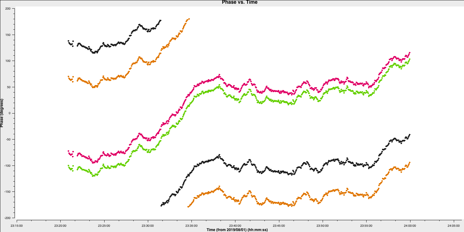
Some things to note here:
- On the 20-30s timescales, we have trackable phase fluctuations caused by the atmosphere, which cause the phases to drift.
- These fluctuations are similar across each spw, indicating that the atmosphere affects our frequency range equally (meaning that we could fix the delay and combine spw for higher S/N solutions).
- The delays are causing absolute phase offsets between the spectral windows, but crucially, these do not appear to change with time (otherwise the gap between the spectral windows would change with time). Because of this, it is suitable to select a long solution interval (e.g., 600 s in this case) for the delay calibration to maximise the S/N of our solutions.
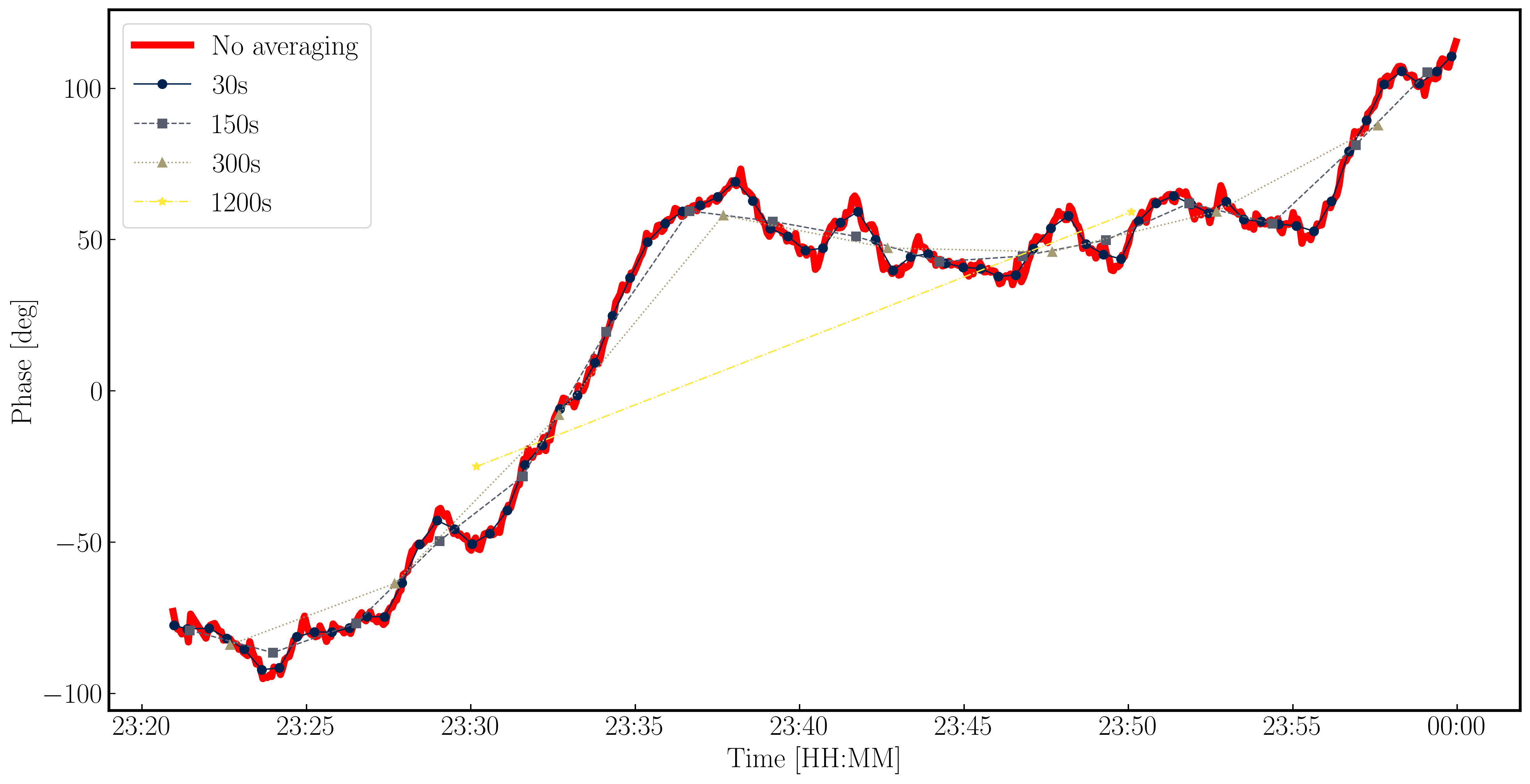
While we have decided on a solution interval for delays, we need to do the same for the phase term. In the plot below, we have overplotted the phase using different averaging intervals for a single spectral window. You can see that we start to lose the general trends caused by the atmosphere when the averaging is too severe. However, we can also see that there's negligible thermal noise on an integration-to-integration basis, so we could actually use a very short solution interval, such as the 30s shown in the plot. This would track the atmospheric fluctuations well.
2B. Pre-bandpass calibration (step 13)
With our solution intervals in hand, we are now going to conduct the gain calibration to isolate the bandpass corrections. This will allow us to calibrate out the atmosphere, clock errors, etc., which change our amplitudes and phases over time.
- Again, for this step, it is advisable to copy and paste your tasks directly into CASA to perform each calibration step bit by bit. If you encounter syntax errors, remember that the variables
gui = Trueandantref = 'Mk2'should have been set in CASA. - Have a look at step 13. We shall begin by calibrating the delays using the CASA task
gaincal. We saw from the figure in the previous section that the absolute offset between the phases of different spws remained almost the same; hence, the delay calibration did not change much (so a long solution interval can be used). Fill in the missing code to generate the delay solutions for the bandpass calibrator. Remember to usehelp(gaincal)!gaincal(vis='all_avg.ms', gaintype='**', field='**', caltable='bpcal.K', spw='0~3',solint='**', refant=antref, refantmode='strict', minblperant=2, minsnr=2)
The gaincal task will generate a calibration table (named bpcal.K in this case) that includes the delay solutions. When applied to the visibilities, these will remove the phase slope versus frequency we saw earlier. However, we always want to plot the solutions to ensure they are reasonable. Good solutions are normally smoothly varying without jumps.
- Take a look at the next
plotmscommand, then enter it into CASA.plotms(vis='bpcal.K', xaxis='time', yaxis='delay', gridrows=3,gridcols=2, iteraxis='antenna', coloraxis='spw', xselfscale=True, yselfscale=True, plotfile='', showgui=gui, overwrite=True)
This should produce a plot like the one shown below.
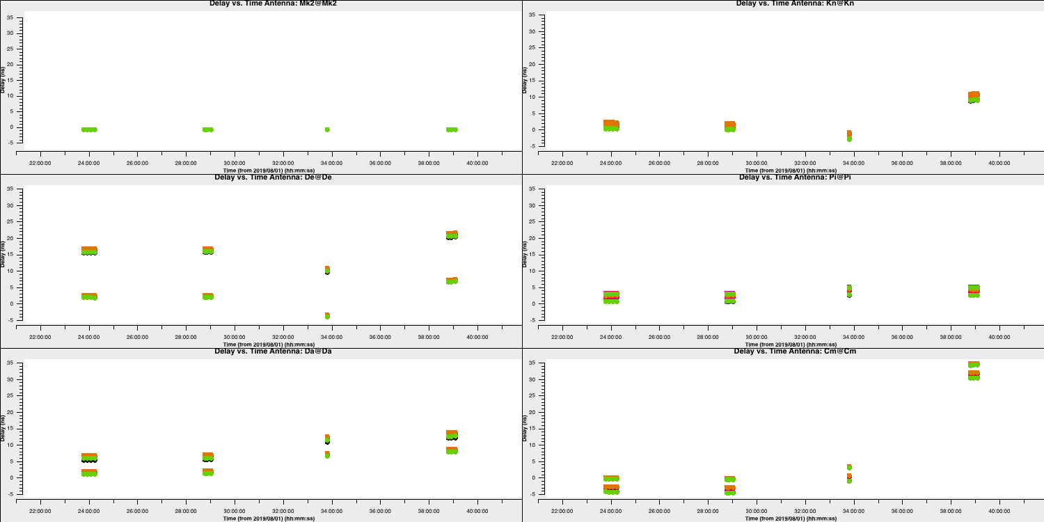
As you can see, the solutions are smooth and generally follow each other. Note the large delay correction for the Cm telescope in the last scan. We saw this in Section 4A, where we plotted amplitude decorrelation by averaging the channels. The huge delay (shown by rapid phase wrapping) corresponds to the 35ns solutions for this scan on this telescope.
With the delay calibration for 0319+4130 complete, the offsets between the spectral windows in the frequency domain have been removed, and we can now concentrate on the time-dependent phase calibration, which will remove the effect of the atmosphere along our line-of-sight to the source.
- Take a look at the second
gaincalcommand and enter the parameters to perform a phase-only calibration of the bandpass calibrator. Note that we include the delay calibration table in thegaintableparameter. CASA performs calibration on the fly, so the delay table will be applied to the visibilities before the phase calibration is solved for.gaincal(vis='all_avg.ms', calmode='**', field='**', caltable='bpcal_precal.p1', solint='**', refant=antref, refantmode='strict', minblperant=2, gaintable=['bpcal.K'], minsnr=2) - Again, we want to plot the solutions to ensure they are not just noise.
	plotms(vis='bpcal_precal.p1',
	       xaxis='time',
	       yaxis='phase',
	       gridrows=3,gridcols=2,
	       iteraxis='antenna', coloraxis='spw',
	       xselfscale=True,
	       yselfscale=True,
	       plotfile='',
	       showgui=gui, overwrite=True)
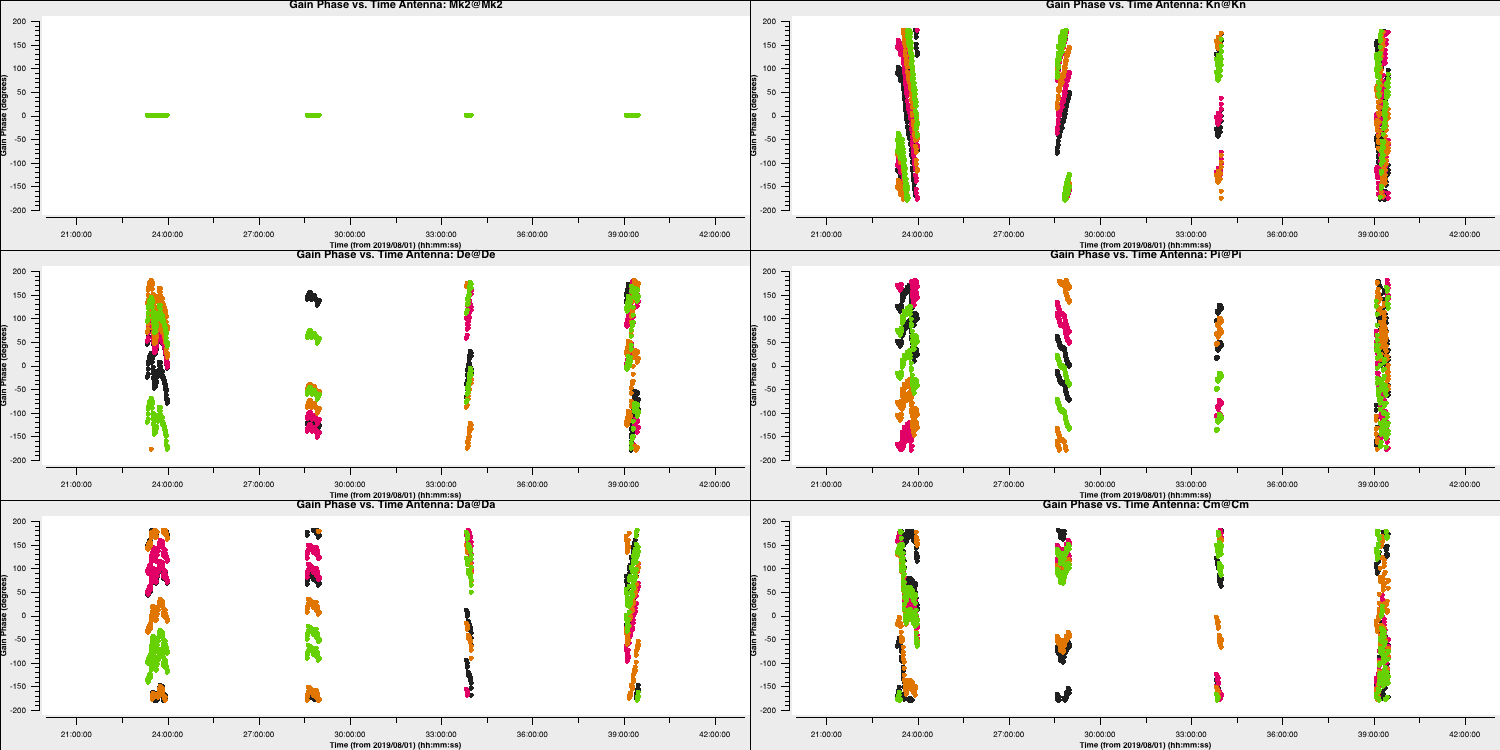
These solutions look great (I used a 30s interval) and seem to follow the phases (and fluctuation timescales) we had seen before. Finally, we have one calibration step missing. We've done delays and phases, and it's just amplitudes that are left.
- Look at the final
gaincalcommand and enter the correct parameters for amplitude-only calibration of the calibrator. You will need to specify thegaintableparameter this time. Note that we did not discuss the amplitude solution interval, but amplitudes typically change more slowly than phases and require a higher S/N for good solutions (see 'closure amplitudes'). In this case, we will use 120s.gaincal(vis='all_avg.ms', calmode='**', field='**', caltable='bpcal_precal.a1', solint='120s', solnorm=False, refant=antref, refantmode='strict', minblperant=2, gaintable=['**','**'], minsnr=2) - Finally, we want to plot these solutions to ensure they look OK and are not noisy.
	plotms(vis='bpcal_precal.a1',
	       xaxis='time',
	       yaxis='amp',
	       gridrows=3,gridcols=2,
	       iteraxis='antenna', coloraxis='spw',
	       xselfscale=True,
	       yselfscale=True,
	       plotfile='',
	       showgui=gui, overwrite=True)
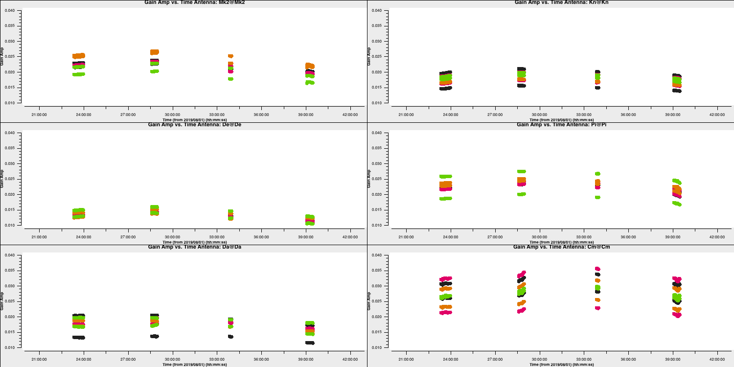
These solutions look good. Note that the amplitudes are very low, and this is because we have rescaled the visibilities to the flux density we set at the start of this section. We will do the same later for the other sources whose true flux densities we don't know.
2C. Derive bandpass solutions (step 14)
With all other corruptions now addressed through the three calibration tables we have derived, the final step is to derive the bandpass calibration table using a special task called bandpass.
- Take a look at step 14, enter the correct parameters for the bandpass calibration, and then enter this at the CASA prompt.
	bandpass(vis='all_avg.ms',
			 caltable='bpcal.B1',
			 field='**',
			 fillgaps=16,
			 solint='inf',combine='scan',
			 solnorm='**',
			 refant=antref,
			 bandtype='B',
			 minblperant=2,
			 gaintable=['**','**','**'],
			 minsnr=3)
You may encounter a few complaints about failed solutions, but these should be directed to the end channels that are flagged anyway.
- Inspect the solutions using the
plotmscommands at the end of Step 14.
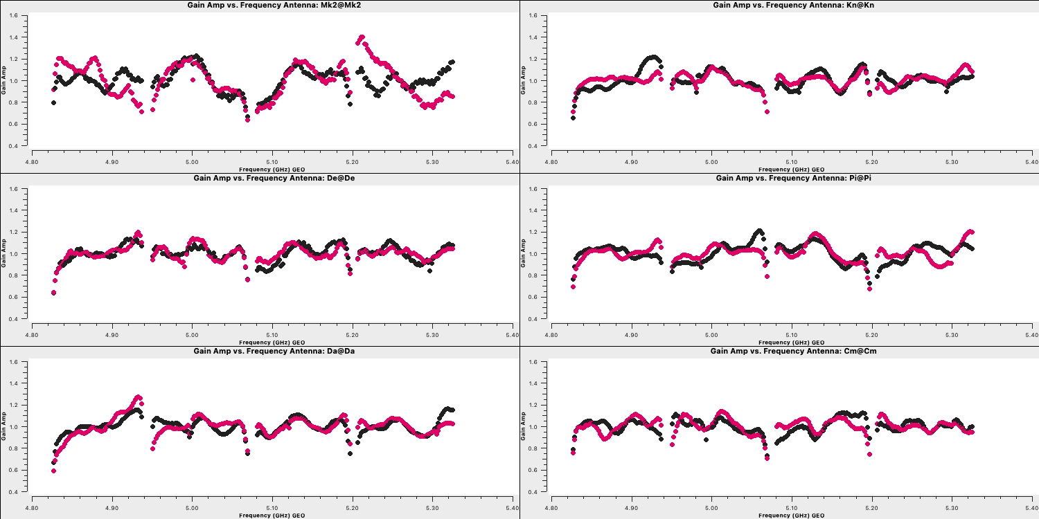
for amplitude and,plotms(vis='bpcal.B1', xaxis='freq', yaxis='amp', gridrows=3,gridcols=2, iteraxis='antenna', coloraxis='corr', xselfscale=True, yselfscale=True, plotfile='', showgui=gui, overwrite=True)
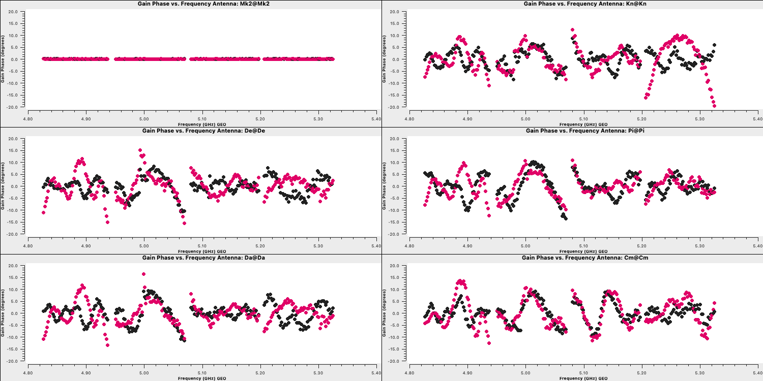
for phase.plotms(vis='bpcal.B1', xaxis='freq', yaxis='phase', gridrows=3,gridcols=2, iteraxis='antenna', coloraxis='corr', xselfscale=True, yselfscale=True, plotfile='', showgui=gui, overwrite=True)
These should produce plots like those below, which correct for the receiver response on each antenna (note the close match to the plots when we flagged the edge channels). This error is antenna-based and direction-independent, so we can apply it to all other sources, as it should not change with time. Note that the spectral index of this source is taken into account here, as it was specified in step 3A (normally you'd do the bandpass calibration twice, with the second time using an estimate of the spectral index).
3. Time-dependent delay calibration (15)
We've calibrated the bandpass calibrator to obtain the bandpass corrections. We now need to derive the time-dependent phase and amplitude corrections for all the calibrators simultaneously. This will allow us to perform phase referencing (as discussed in the lecture) so we can observe the target source. As before, we will start with the delays and then move on to the phase and amplitude corrections.
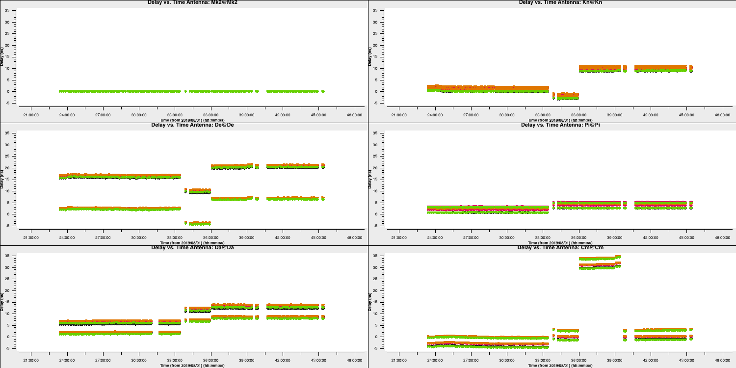
- Review step 15 and enter the parameters for both the gaincal and plotting commands to perform delay calibration for all calibrator sources. The solution interval used for the bandpass calibrator should be applicable here as well. Remember to apply the bandpass calibration table now.
gaincal(vis='all_avg.ms', gaintype='K', field='**', caltable='all_avg.K', spw='0~3',solint='**', refant=antref, refantmode='strict', gaintable=['**'], minblperant=2, minsnr=2) plotms(vis='all_avg.K', xaxis='**', yaxis='**', gridrows=3,gridcols=2, iteraxis='antenna', coloraxis='spw', xselfscale=True, yselfscale=True, plotfile='', showgui=gui, overwrite=True) - Once you are happy, execute step 15 and review the output of
plotms
You should end up with a plot that looks like the one below. The solutions vary smoothly, with only a few jumps, which shows that our solutions are ok.
3A. Inspect effects of calibration (16)
Important: If you are short on time, skip this step and just read the information and plots shown here.
In this step, we shall apply the delay and bandpass solutions to the calibration sources as a test to verify that they produce a flat bandpass for the phase-reference source (not on the fly this time!). There is no need to apply the time-dependent calibration, as we have not derived it for the phase-reference source yet anyway.
To apply these, we shall use a task called applycal. Some notes on applycal:
- The first time
applycalis run, it creates a CORRECTED data column in the MS, which is quite slow. - Each time
applycalis run, it replaces the entries in the CORRECTED column, i.e. the corrected column is not cumulative, but you can giveapplycala cumulative list of gain tables. applymodecan be used to flag data with failed solutions but we do not want that here as this is just a test.- The
interpparameter can take two values for each gaintable to be applied, the first determining interpolation in time and the second in frequency. The times of data to be corrected may coincide with, or be bracketed by the times of calibration solutions, in which caselinearinterpolation can be used, the default, normally used if applying solutions derived from a source to itself, or from phase ref to target in alternating scans. However, if solutions are to be extrapolated in time from one source to another which are not interleaved, then nearest is used. A similar argument covers frequency. There are additional modes not used here (seehelp(applycal)).
- Fill in the
applycalstep in step 16, then look at the followingplotmscommand, which will plot the 'before and after' phase reference phase and amplitude against frequency.applycal(vis='all_avg.ms', field='1302+5748,0319+4130,1331+3030', calwt=False, applymode='calonly', gaintable=['**','**'], interp=['**','**,**']) - Execute step 16, then take a look at the plots saved to the current directory.
The plot below shows the uncorrected and corrected amplitudes and phases for the Mk2-Cm baseline of the phase reference source (1302+5748), with data coloured by scan. It has been replotted in Python for clarity.
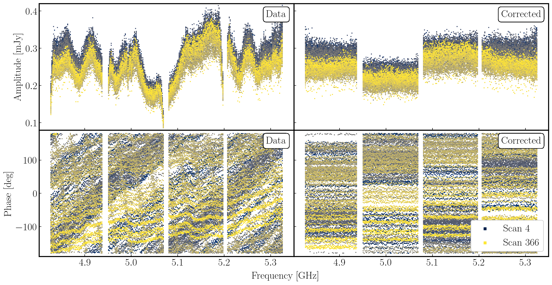
In the figure, each scan is coloured separately and shows random phase offsets and amplitude discrepancies compared with other scans, but within each individual time interval it is quite flat. So we can average in frequency across each spw and plot the data to show any remaining time-dependent errors.
4. Gain calibration (step 17)
4A. Time dependent phase calibration
As with the bandpass calibrator, we now move on to correcting for the phase fluctuations caused by turbulence in the atmosphere. This will allow us to phase-reference and see our target source, as the phase calibrator is approximately along the same line of sight.
- Take a look at step 17 and insert the parameters that will enable us to perform time-dependent phase calibration of all calibrator sources.
gaincal(vis='all_avg.ms', calmode='p', caltable='calsources.p1', field='**,**,**', solint='**', refant=antref, refantmode='strict', minblperant=2,minsnr=1, gaintable=['all_avg.K','bpcal.B1'], interp=['linear','nearest,nearest']) - Copy this into the CASA prompt, run it to generate the calibration table, and have a look at the logger.
The logger should show something like this (if you used 16s solution intervals, like me):
2022-08-12 10:08:20	INFO		Writing solutions to table: calsources.p1
2022-08-12 10:08:21	INFO	calibrater::solve	Finished solving.
2022-08-12 10:08:21	INFO	gaincal::::casa	Calibration solve statistics per spw:  (expected/attempted/succeeded):
2022-08-12 10:08:22	INFO	gaincal::::casa	  Spw 0: 1988/1572/1571
2022-08-12 10:08:22	INFO	gaincal::::casa	  Spw 1: 1988/1572/1571
2022-08-12 10:08:22	INFO	gaincal::::casa	  Spw 2: 1988/1572/1571
2022-08-12 10:08:22	INFO	gaincal::::casa	  Spw 3: 1988/1572/1571
This means that although there are 1988 16s intervals in the calibration sources' data, about a fifth (1988-1572=416) of them have been partially or fully flagged. But almost all (99.93%) of the intervals that do have enough unflagged ('attempted') data gave good solutions ('succeeded'). There are no further messages about completely flagged data, but in the terminal you see a few messages when there are fewer than the requested 2 baselines per antenna unflagged.
Found no unflagged data at:   (time=2019/08/02/21:00:04.5 field=0 spw=3 chan=0)
 Insufficient unflagged antennas to proceed with this solve.
   (time=2019/08/02/21:17:19.2 field=0 spw=3 chan=0)
Here, there are very few predictable failures. If there are many or unexpected failures, investigate - perhaps there are unflagged bad data, pre-calibration has not been applied, or an inappropriate solution interval was used.
- Plot the solutions, and you should get something that tracks the phases well (as shown below).
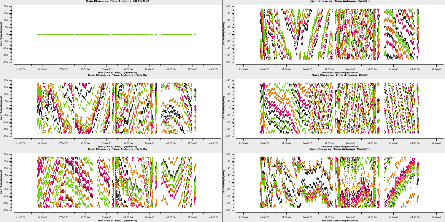
4B. Time dependent amplitude calibration
Next, we are going to derive time-dependent amplitude solutions for all the calibration sources, applying the delay, bandpass, and time-dependent phase solution tables.
- Take a look at the second
gaincalentry in step 17, and insert a suitable solution interval, the tables to apply, and interpolation modes. Note that if you set a solint longer than a single scan on a source, the data will still be averaged only within each scan unless an additional 'combine' parameter is set (not needed here).gaincal(vis='all_avg.ms', calmode='a', caltable='calsources.a1', field='**,**,**', solint='**', solnorm=False, refant=antref, minblperant=2,minsnr=2, gaintable=['**','**','**'], interp=['linear','nearest,nearest','**']) - The logger shows a similar proportion of expected/attempted solution intervals to that for phase, but those with failed phase solutions are not attempted, so all attempted solutions work. Plot these solutions to ensure they look ok.
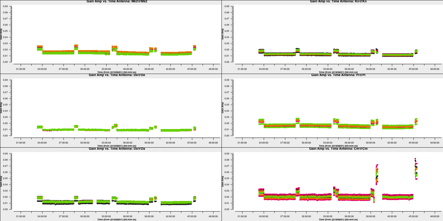
The plot above shows the time-dependent amplitude solutions for the L polarisation only, coloured by spw. The solutions for each source look similar, but there are significant differences between sources, since they have all (apart from 1331+3030 and 0319+4130) been compared with a 1 Jy model, yet they have different flux densities.
5. Determining true flux densities of other calibration sources (steps 18-19)
The solutions for 1331+3030 in calsources.a1 include the correct scaling factor to convert the raw correlator units to Jy and remove time-dependent errors. This is used to calculate the scaling factor for the other calibration sources in the CASA task fluxscale. We run this task differently because the calculated fluxes are returned as a Python dictionary. They are also written to a text file. Only the best data are used to derive the flux densities, but the output is valid for all antennas. This method assumes that all sources without starting models are point sources, so it cannot be used for an extended target.
- We are not going to input anything for step 18, so just run it and we shall look at the outputs.
	os.system('rm -rf calsources.a1_flux calsources_flux.txt')
	calfluxes=fluxscale(vis='all_avg.ms',
						caltable='calsources.a1',
						fluxtable='calsources.a1_flux',
						listfile='calsources_flux.txt',
						gainthreshold=0.3,
						antenna='!De',      # Least sensitive
						reference='1331+3030',
						transfer=phref)
If you type calfluxes after the step has been run, it will show you the Python dictionary.
The individual spw estimates may have uncertainties of up to $\sim20\%$, but the bottom lines give the fitted flux density and spectral index for all spw, which should be accurate to a few per cent. These require an additional scaling of 0.938 to account for the resolving out of flux of 1331+3130 by e-MERLIN. The Python dictionary calfluxes is edited to apply this:
	eMcalfluxes={}
	for k in calfluxes.keys():
		if len(calfluxes[k]) > 4:
			a=[]
			a.append(calfluxes[k]['fitFluxd']*eMfactor)
			a.append(calfluxes[k]['spidx'][0])
			a.append(calfluxes[k]['fitRefFreq'])
			eMcalfluxes[calfluxes[k]['fieldName']]=a
Next, we use setjy in a loop to set the flux densities for each calibration source. The logger will report the values being set.
	for f in eMcalfluxes.keys():
		setjy(vis='all_avg.ms',
			  field=f,
			  standard='manual',
			  fluxdensity=eMcalfluxes[f][0],
			  spix=eMcalfluxes[f][1],
			  reffreq=str(eMcalfluxes[f][2])+'Hz')
The default in setjy is to scale by the spectral index for each channel. Finally, we plot the models for the bandpass calibrators, amplitude against frequency, to see the spectral slopes.
	plotms(vis='all_avg.ms', field=phref, xaxis='frequency',
		   yaxis='amp',ydatacolumn='model',
		   coloraxis='spw',correlation='RR',
		   customsymbol=True,symbolshape='circle', symbolsize=5,
		   showgui=gui,overwrite=True,
		   plotfile='phref_model.png')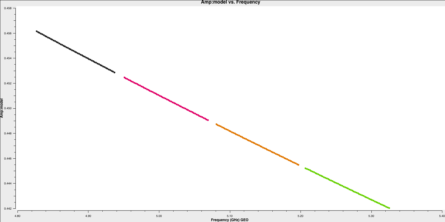
- Move on to step 19, review the inputs, and run the step. Again, we won't be inputting parameters here. We are now going to use these newly found flux densities to scale our visibilities to the correct physical values using an amplitude correction.
	gaincal(vis='all_avg.ms',
			calmode='a',
			caltable='calsources.a2',
			field=calsources,
			solint='inf',
			refant=antref,
			minblperant=2,minsnr=2,
			gaintable=['all_avg.K','bpcal.B1','calsources.p1'],
			interp=['linear','','linear'])

	# Plot solutions
	plotms(vis='calsources.a2',
	       xaxis='time',
	       yaxis='amp',
	       gridrows=3,gridcols=2,
	       iteraxis='antenna', coloraxis='spw',
	       xselfscale=True,
	       yselfscale=True,
	       showgui=gui,overwrite=True,
	       plotfile='calsources.a2.png')
This should produce a plot that is shown below:
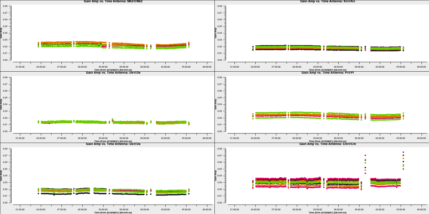
You expect to see a similar scaling factor across all sources. 1331+305 is somewhat resolved, yielding slightly higher values for Cm (the antenna providing the longest baselines).
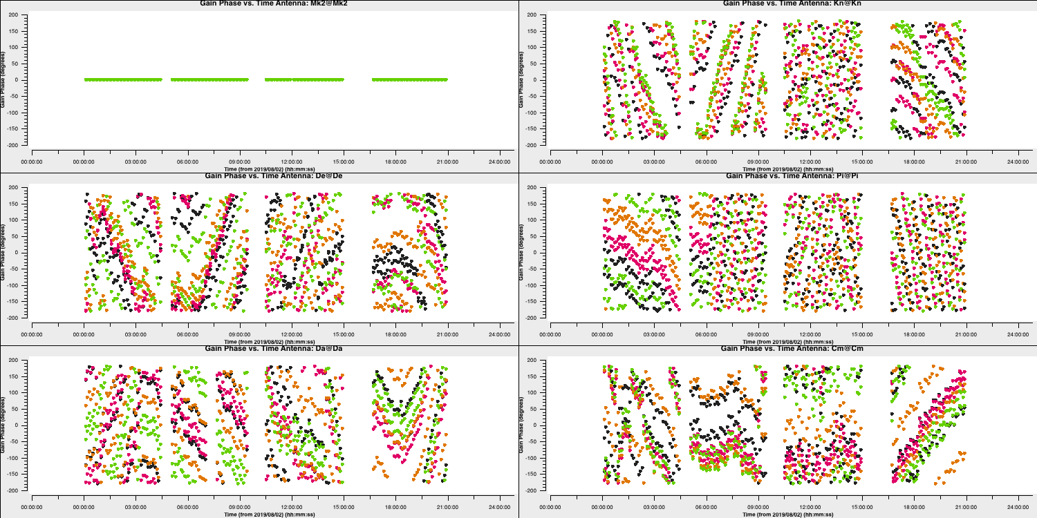
In the final part of the section, we are going to derive phase solutions again, this time combining all data on the phase calibrator source. This is because we only need one solution to interpolate across the target scans. We derive these and plot them with the following code.
	gaincal(vis='all_avg.ms',
			calmode='p',
			caltable='phref.p2',
			field=phref,
			solint='inf',
			refant=antref,
			refantmode='strict',
			minblperant=2,minsnr=2,
			gaintable=['all_avg.K','bpcal.B1'],
			interp=['linear',''])

	# Plot solutions
	plotms(vis='phref.p2',
	       xaxis='time',
	       yaxis='phase',
	       gridrows=3,gridcols=2,
	       iteraxis='antenna', coloraxis='spw',
	       xselfscale=True,
	       yselfscale=True,
	       showgui=gui,overwrite=True,
	       plotfile='phref.p2.png')
	os.system('mv phref.p2?*.png phref.p2.png')
This should produce a plot like the one shown below:
6. Apply solutions to target (steps 20-21)
- Look at and execute step 20 while reading the following information about this step.
This step applies the bandpass correction to all sources. For the other gaintables, for each calibrator (field), the solutions for the same source (gainfield) are applied. gainfield='' for the bandpass table means applying solutions from all fields in that gaintable. applymode='calflag' flags data with failed solutions, which is ok, as we know these were due to bad data. We use a loop over all calibration sources.
	cals=bases
	cals.remove(target)
	for c in cals:
		applycal(vis='all_avg.ms',
				 field=c,
				 gainfield=[c, '',c,c],
				 calwt=False,
				 applymode='calflag',
				 gaintable=['all_avg.K','bpcal.B1','calsources.p1','calsources.a2'],
				 interp=['linear','nearest','linear','linear'],
				 flagbackup=False)
We then apply the phase-ref solutions to the target. We assume that the phase-reference scans bracket the target scans, so linear interpolation is used except for bandpass.
	applycal(vis='all_avg.ms',
			 field='1252+5634',
			 gainfield=['1302+5748','','1302+5748','1302+5748'],
			 calwt=False,
			 applymode='calflag',  # Not too many failed solutions -  OK to flag target data
			 gaintable=['all_avg.K','bpcal.B1','phref.p2','calsources.a2'],
			 interp=['linear','nearest','linear','linear'],
flagbackup=True) plotms(vis='all_avg.ms', field='1302+5748', xaxis='uvdist',
yaxis='amp',ydatacolumn='corrected',
avgchannel='64',correlation='LL,RR',coloraxis='spw',
overwrite=True, showgui=gui,
plotfile='1302+5748_amp-uvdist.png')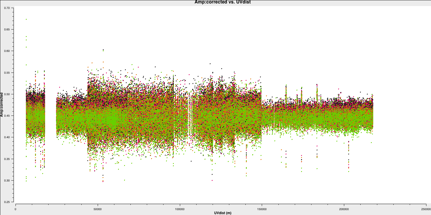
This looks quite point-like. Let's repeat the above for the target.
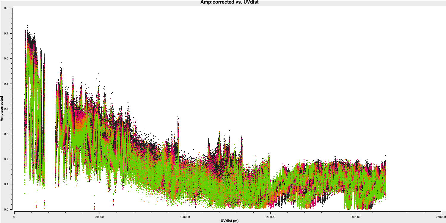
Hurray, there's some structure here.
As a test, QUESTION 5: What do the plots of amplitude against $uv$ distance tell you?
The amplitudes are noisiest out to 130 km, as these are the Defford baselines, which are less sensitive. There is a little data that is anomalously low, but this is ok as the target is bright.
The target has higher amplitudes on shorter baselines, indicating structure on scales larger than 50 mas, and complex structure on the long baselines.
Finally, in step 21, we will split out the target source.
	mstransform(vis='all_avg.ms',
										field='1252+5634',
										correlation='LL,RR',
										outputvis='1252+5634.ms',
										keepflags=False,
										usewtspectrum=True,
										timeaverage=True,
										timebin='16s',
										chanaverage=True,
										chanbin=4)
- Execute step 21.
The task mstranform will create a new measurement set called 1252+5634.ms that contains the calibrated visibilities of the target source (moving the CORRECTED data to the DATA column in the new measurement set). This means we don't need to apply those tables on the fly during further calibration. We have also specified some averaging so that the next steps of the tutorial can be processed more quickly. In step 21, you will see that another listobs is run to look at the data, and we have phase-rotated the data to make the imaging steps easier. If you wish to have more information on this, ask your tutor.
This concludes the calibration section. Make sure you save 1252+5634.ms for the imaging and self-calibration tutorials.
Congratulations, you have finished the second part of this tutorial and calibrated your data. Next, we shall move on to imaging your objects. Follow the link below to continue.