Advanced imaging
Data required
For this section, you want to download the fully self-calibrated data set, contained in the tar bundle ERIS26_adv_imaging.tar.gz. This data set has had the CORRECTED self-calibrated visibilities split into the DATA columns of this measurement set (to reduce the data size), and the most recent self-calibration model has been Fourier transformed into the measurement set (creating a MODEL column).
You also want to copy the two calibration scripts we have been using for the previous imaging and self-calibration tutorial. However, we have included copies of these scripts in the tar bundle. Ensure that you have the following in your folder,
1252+5634_adv_im.ms- fully self-calibrated visibilities.3C277.1_imaging_outline2026.py- imaging script.3C277.1_imaging_all2026.py- cheat script containing the answers.
Table of contents
1. Reweigh the data according to sensitivity (step 13)
Often, especially for heterogeneous arrays, the assigned weighting is not optimal for sensitivity. For example, the Cambridge (Cm) telescope is more sensitive; therefore, to obtain the optimal image, it must be given a larger weight than the other arrays.
To recalculate the optimal weights, we use the task statwt, which calculates the weights based on the scatter in small samples of data. Note that the original data are overwritten, so you might want to copy the MS to a different name or directory first.
There are a lot of options here, but we are just going to use the default options. You can try different weightings if you'd like.
- Take a look at step 13, where you will see three commands. The
plotmsstep will plot the weights before and after, while thestatwtcommand will rescale them. Note that we are going to use the residual column to estimate the scatter (which is the data $-$ model column).statwt(vis='**', datacolumn='residual_data') - Enter the relevant parameters (remembering that we are using a different measurement set) and execute step 13.
- Take a look at the
plotmsresults.
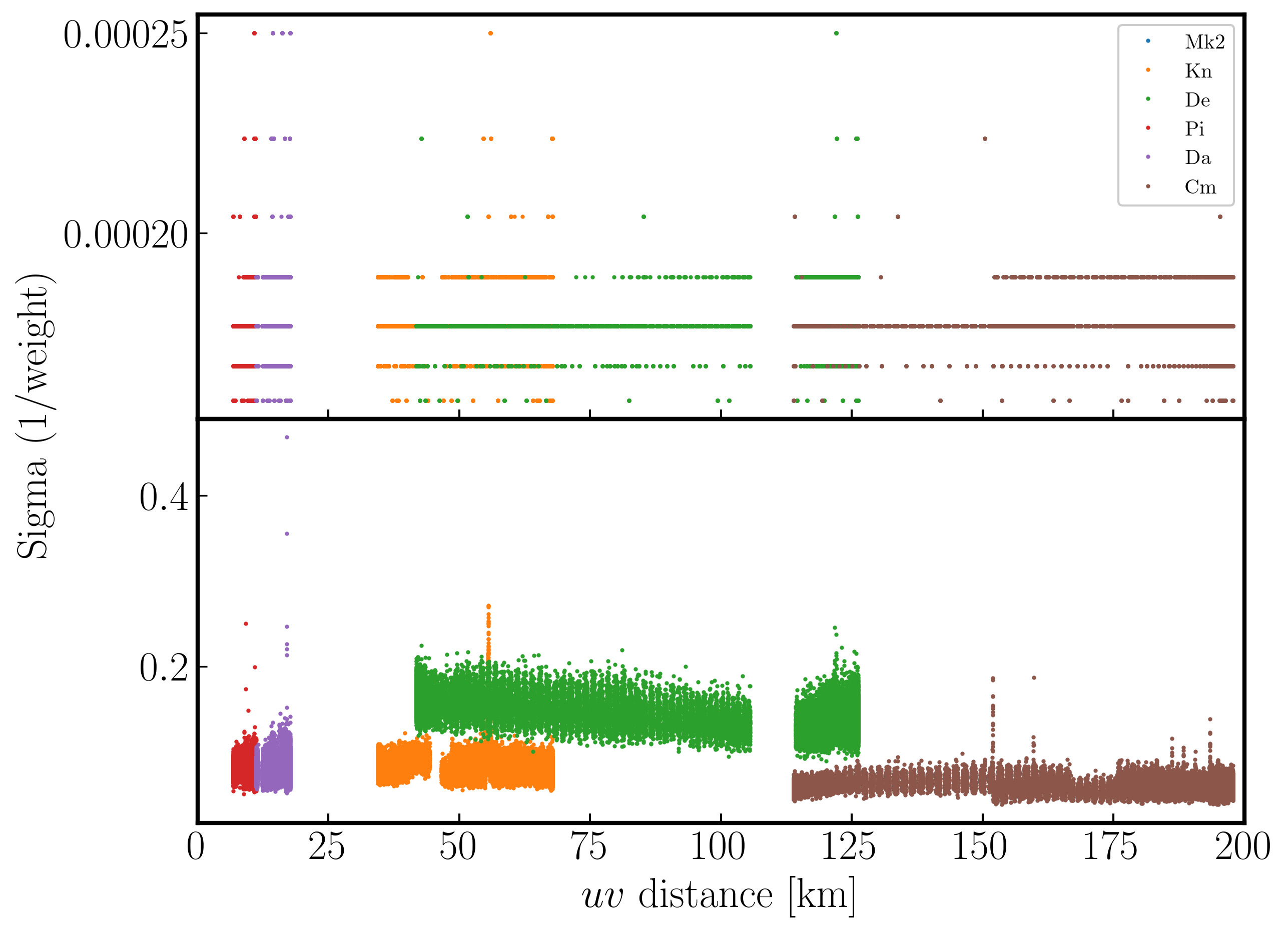
In the plot below, we show the weights before (top panel) and after re-weighting (bottom panel) for the baselines to our reference antenna (Mk2). As you can see, the telescopes have similar weights despite Cm being more sensitive. With the use of statwt, the weights now reflect the sensitivities, with Cm having the lowest sigma weight, so it is more sensitive.
2. Try multi-scale clean (step 14)
Let's image the re-weighted data using multiscale clean, which assumes that the sky can be represented by a set of Gaussians rather than delta functions.
- Look at step 14 and enter the imaging parameters for multi-scale clean. Have a look at the help for the
tcleantask, which suggests suitable values for thescaleparameter.Linuxtclean(vis=target+'_adv_im.ms', imagename='advIMmulti', imsize=['**','**'], cell='**arcsec', specmode='mfs', niter=3000, cycleniter=300, gain=0.2, threshold=0, deconvolver='mtmfs', scales=['**','**','**'], nterms=2, interactive=True)Mac OSiclean(vis=target+'_adv_im.ms', imagename='advIMmulti', imsize=['**','**'], cell='**arcsec', specmode='mfs', niter=3000, cycleniter=300, gain=0.2, threshold=0, deconvolver='mtmfs', scales=['**','**','**'], nterms=2)rmsmulti=imstat(imagename='advIMmulti.image.tt0', box='**,**,**,**')['rms'][0] peakmulti=imstat(imagename='advIMmulti.image.tt0', box='**,**,**,**')['max'][0] print('advIMmulti.image.tt0 rms = %7.3f mJy/bm' % (rmsmulti*1000.)) print('advIMmulti.image.tt0 peak = %7.3f mJy/bm' % (peakmulti*1000.)) print('advIMmulti.image.tt0 S/N = %7.3f' % (peakmulti/rmsmulti)) - Once you are happy, execute step 14 and deconvolve the image.
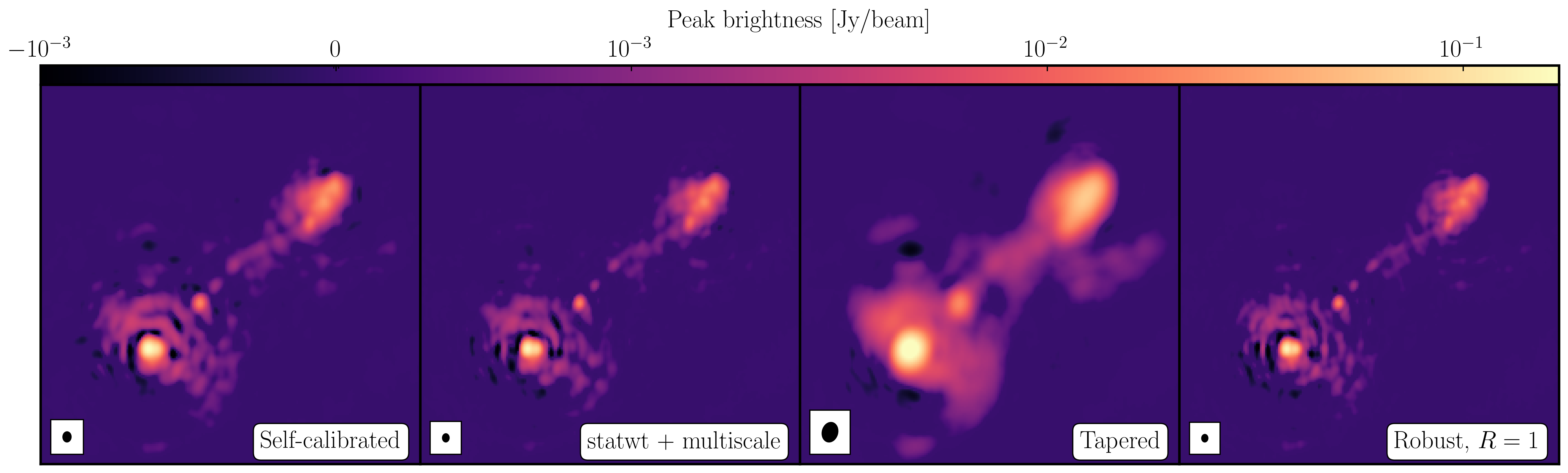
You will find that the beam is now slightly smaller (I got $52\times42\,\mathrm{mas}$) because the longer baselines have more weight, so the peak is lower. I got $S_p \sim 149.235 \,\mathrm{mJy\,beam^{-1}}$ and $\sigma \sim 50\,\mathrm{\mu Jy\,beam^{-1}}$ when using a scales=[0,2,5]. Note that this gives a lower S/N despite the optimal reweighting. This is mainly because the beam area is smaller, so the peak flux in beam area units is lower.
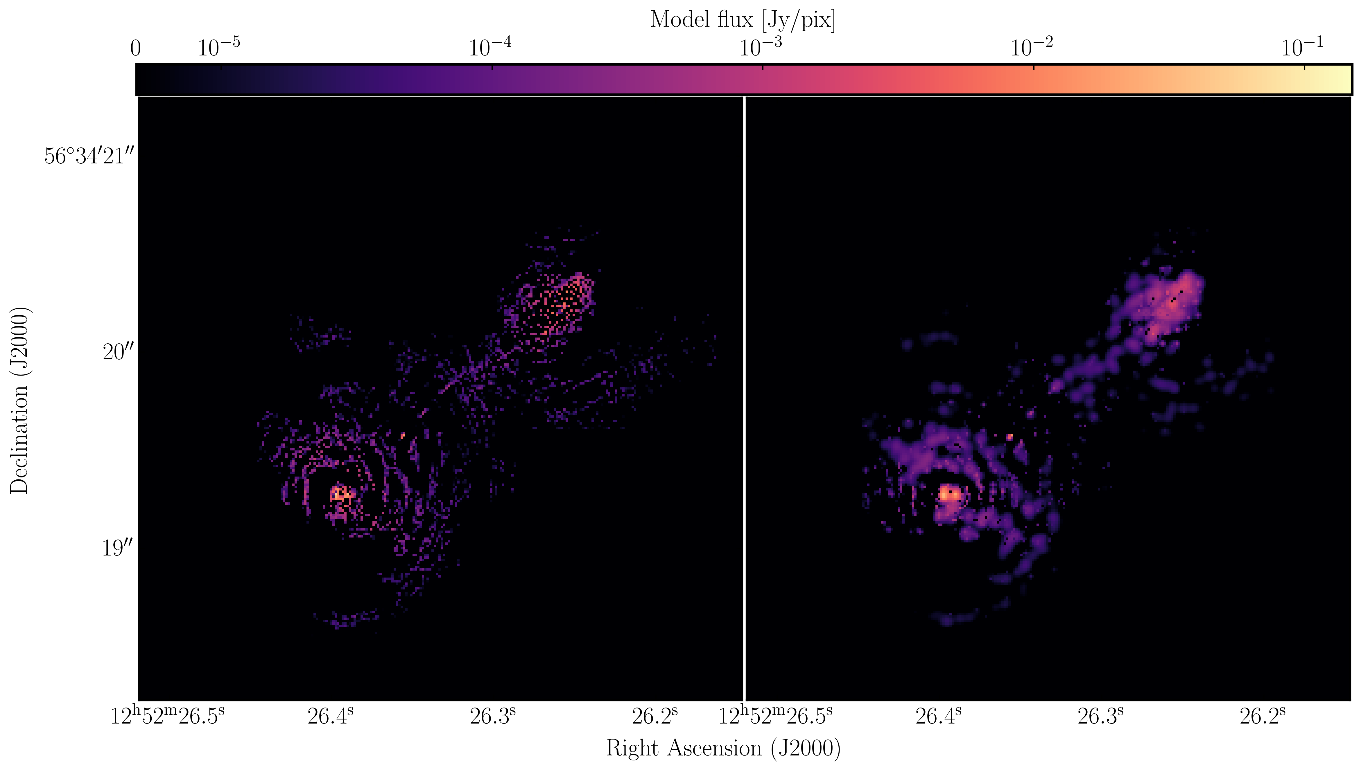
With multi-scale CLEAN, we can compare the two models to see the difference between them. Multi-scale CLEAN is often required when diffuse emission dominates, and it can then be used to improve the self-calibration model. Below, I have plotted the models using standard delta-function CLEAN and multi-scale CLEAN.
3. Taper the visibilities during imaging (step 15)
Next, we shall experiment with changing the relative weights given to longer baselines. Applying a taper reduces this, yielding a larger synthesised beam that is more sensitive to extended emission. This only changes the weights during gridding for imaging, with no permanent change to the uv data. However, strong tapering increases the noise.
- Look at the $uv$ distance plot and choose an outer taper (a half-power Gaussian taper applied to the data) that is about 2/3 of the longest baseline. Units are wavelengths, so calculate that or plot amplitude vs. $uv$ wave.
- Enter this and the imaging parameters into step 15, then execute.
Linux
	tclean(vis=target+'_adv_im.ms',
		   imagename='advIMtaper',
		   imsize=['**','**'],
		   cell='**arcsec',
		   specmode='mfs',
		   niter=4000,
		   cycleniter=300,
		   gain=0.2,
		   threshold=0,
		   deconvolver='mtmfs',
		   uvtaper=['**Mlambda'],
		   scales=[0],
		   nterms=2,
		   interactive=True)
Mac OSiclean(vis=target+'_adv_im.ms', imagename='advIMtaper', imsize=['**','**'], cell='**arcsec', uvtaper=['**Mlambda'], specmode='mfs', niter=4000, cycleniter=300, gain=0.2, threshold=0, deconvolver='mtmfs', scales=[0], nterms=2)rmstaper=imstat(imagename='advIMtaper.image.tt0', box='**,**,**,**')['rms'][0] peaktaper=imstat(imagename='advIMtaper.image.tt0', box='**,**,**,**')['max'][0] - Inspect the image, check the beam size and the image statistics.
For a taper of 2.5 Mlambda, I obtained a restoring beam size of $129\times100\,\mathrm{mas}$, a peak brightness of $S_p \sim 265.595\,\mathrm{mJy\,beam^{-1}}$ and an rms noise of $\sigma \sim 78\,\mathrm{\mu Jy\,beam^{-1}}$.
4. Different imaging weights: Briggs robust (step 16)
In our final imaging experiments, we shall adjust the relative weights given to longer baselines. Default natural weighting gives zero weight to parts of the $uv$ plane with no samples. Briggs weighting interpolates between samples, giving more weight to interpolated areas for lower values of robust. For an array like e-MERLIN with sparser sampling on long baselines, this increases their contribution, i.e., making the synthesised beam smaller. This may bring out the jet/core in more detail, at the expense of the extended lobes. Low values of robust increase the noise. You can combine with tapering or multiscale, but initially remove these parameters.
- Take a look at step 16 and enter the parameters to perform imaging with Briggs weighting and a robust value of 1. Remember to use the help function to find the correct inputs.
Linux
	tclean(vis=target+'_adv_im.ms',
		   imagename='advIMrobust',
		   imsize=['**','**'],
		   cell='**arcsec',
		   specmode='mfs',
		   niter=4000,
		   cycleniter=300,
		   gain=0.2,
		   threshold=0,
		   deconvolver='mtmfs',
		   nterms=2,
		   weighting='**',
		   robust='**',
		   interactive=True)
Mac OSiclean(vis=target+'_adv_im.ms', imagename='advIMrobust', imsize=['**','**'], cell='**arcsec', specmode='mfs', niter=4000, cycleniter=300, gain=0.2, threshold=0, deconvolver='mtmfs', nterms=2, weighting='**', robust='**')rmsrobust=imstat(imagename='advIMrobust.image.tt0', box='**,**,**,**')['rms'][0] peakrobust=imstat(imagename='advIMrobust.image.tt0', box='**,**,**,**')['max'][0] - Once you are done, execute and clean the image.
- If you have time, you can also experiment with other robust values and weighting schemes.
With a robust parameter of 1, I produced an image with a restoring beam of $48\times39\,\mathrm{mas}$, $S_p \sim 143.404\,\mathrm{mJy\,beam^{-1}}$ and $\sigma \sim 52\,\mathrm{\mu Jy\,beam^{-1}}$
5. Summary and conclusions
This tutorial investigated the various imaging techniques which can be used to enhance features. In the first instance, we used statwt to optimally reweight the data to maximise sensitivity. We find that the Cm telescope is the most sensitive (as it is 32m wide) and contains all the long baselines. As a result, these long baselines are more prominent in the image, producing a higher-resolution image than we've seen before. However, the peak flux decreases, and so does the sensitivity! In addition, we used multiscale clean to better deconvolve the large, fluffy structures which standard clean can struggle with.
The next step we took was to taper the weights with respect to $uv$ distance. The downweighting of the long baselines means that we are more sensitive to larger structures, hence our resolution is lower. However, because of the sensitivity contained in these long baselines, we have a much larger rms.
Finally, we introduced robust weighting schemes. These schemes provide a clear way to achieve intermediate resolutions between naturally and uniformly weighted data.
| Peak brightness | Noise (rms) | S/N | Beam size | |
|---|---|---|---|---|
| [$\mathrm{mJy\,beam^{-1}}$] | [$\mathrm{mJy\,beam^{-1}}$] | [$\mathrm{mas\times mas}$] | ||
| statwt + multiscale | 148.235 | 0.050 | 2964.7 | 52 $\times$ 42 |
| Tapering | 265.595 | 0.078 | 3405.1 | 129 $\times$ 100 |
| Robust weighting ($R=1$) | 143.404 | 0.052 | 2757.8 | 48 $\times$ 39 |