TW Hya: N₂H⁺ Spectral Line Imaging
Data required
In this tutorial we will image emission from the N₂H⁺ ($J=4-3$) transition in the protoplanetary disc surrounding TW Hya. TW Hya is one of the nearest and best-studied planet-forming discs and has therefore become an important benchmark for studies of disc chemistry and structure.
We shall use self-calibrated ALMA observations from Project 2011.0.00340.S, "Searching for H₂D⁺ in the disk of TW Hya" (PI: Chunhua Qi). These data are also used in the official ALMA imaging tutorials.
The calibrated measurement set and the continuum image can be downloaded using the link below:
Alternatively, you can download and un-tar the data from the command line:
wget https://www.jb.man.ac.uk/ERIS26/data/ERIS26_sp_line_twhya.tar.gz
tar -zxvf ERIS26_sp_line_twhya.tar.gz
After downloading the data, verify that the measurement set is available in your working directory before proceeding.
Table of contents
1. Inspect the data
Before imaging any spectral-line dataset it is important to understand the data. The first step is therefore to inspect the measurement set and determine:
- The science target.
- The number of spectral windows.
- The observing frequency.
- The antenna configuration.
This information will be useful later when choosing imaging parameters.
In CASA
listobs(
vis='twhya.ms',
)
Take a few minutes to inspect the output. In particular, identify:
- The field corresponding to TW Hya.
- The spectral window containing the N₂H⁺ transition.
- The central observing frequency.
- The total number of channels.
These quantities will be needed throughout the reduction process.
2. Determine the channels containing the line feature
Before producing a spectral cube we must determine which channels contain spectral-line emission. We also need to identify channels that are free of line emission because these will later be used to fit and subtract the continuum.
A convenient way to do this is to average the visibilities and plot amplitude as a function of channel number/frequency/velocity (i.e. a spectrum).
In CASA
plotms(
vis='twhya.ms',
xaxis='channel',
yaxis='amp',
field='5',
avgspw=False,
avgtime='1e9',
avgscan=True,
avgbaseline=True,
showgui=True,
)
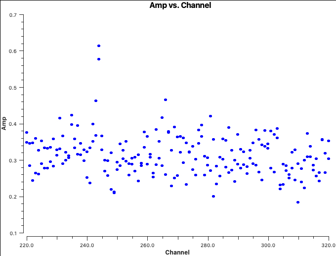
To zoom-in use in plotms window in the Data panel (or you can use it as a command-line input in plotms):
spw='0:220~320'
In CASA
linefree='0:0239;281383'
These line-free channels will form the basis for continuum subtraction done next.
3. Continuum Subtraction
The measured visibilities contain contributions from both continuum emission and line emission.
For many scientific applications we are interested only in the spectral line itself. We therefore fit a continuum model using the line-free channels identified in the previous section and subtract this model directly in the visibility domain.
In CASA
os.system('rm -rf twhya.contsub.ms')

uvcontsub(
vis='twhya.ms',
field='5',
fitspec=linefree,
fitorder=0,
outputvis='twhya.contsub.ms',
)
In CASA
plotms(
vis='twhya.contsub.ms',
xaxis='channel',
yaxis='amp',
field='5',
avgspw=False,
avgtime='1e9',
avgscan=True,
avgbaseline=True,
showgui=True,
)
The continuum-subtracted data should now have an average amplitude close to zero in the line-free channels.
4. Creating a Dirty Cube
Before performing any deconvolution it is often useful to examine the dirty cube.
A dirty cube is produced by Fourier transforming the visibilities without applying any CLEAN iterations. Many of the parameters used for creating a cube are similar to what you used while creating a continuum image. The main difference is, while creating the continuum image you averaged all the channels together. However, here you are going to make an image of each channel (or a few channels averaged together) to obtain a three dimensional data product where the third dimension is the velocity axis.
This allows us to:
- Estimate the image noise.
- Determine which channels contain emission (even the weak emission channels we may have missed in the plotms inspection earlier).
- Decide on an appropriate cleaning strategy.
restoringbeam='common' makes sure that the image of each channel has the same restoring beam.
nchan is the total number of channels in the cube, start is the first channel (either in channel number, frequency or velocity) and width is the channel width. This option can be used to average multiple channels together while making the cube.
The logic behind choosing a few parameters used below such as the 'imsize' and 'cell' are the same as what you learnt in continuum imaging. Can you tell us why the cell and imsize are chosen to have those values?
We use veltype='radio' and outframe='LSRK' for Galactic studies and the rest frequency is simply the transition frequency of the line in question, in this case, the N₂H⁺ line. See the introduction page for an explanation of different velocity types, reference frames and choice of rest frequencies.
In CASA
rstfrq = '372.67249GHz'
In CASA
os.system('rm -rf twhya.dirty.cube*')

tclean(
vis='twhya.contsub.ms',
imagename='twhya.dirty.cube',
field='5',
spw='0',
specmode='cube',
perchanweightdensity=True,
nchan=15,
start='0.0km/s',
width='0.5km/s',
outframe='LSRK',
restfreq=rstfrq,
deconvolver='hogbom',
gridder='standard',
imsize=[250, 250],
cell='0.1arcsec',
weighting='briggsbwtaper',
robust=0.5,
restoringbeam='common',
interactive=False,
niter=0,
pbcor=True
)
5. Inspecting the cube
Check the spatial resolution of the cube, the number of channels, velocity resolution etc.
In CASA
imhead(
imagename='twhya.dirty.cube.image.pbcor'
)
Next, the RMS noise provides a quantitative estimate of the sensitivity of the observations and will guide the choice of stopping threshold during CLEANing.
The imstat task calculates basic statistical properties of an image, including the mean, maximum value and RMS noise.
In CASA
imstat('twhya.dirty.cube.image.pbcor', chans='0~1')
Note down the RMS values provided by imstat.
Now view the dirty cube in CARTA.
In CARTA
Open the dirty cube in CARTA and examine the emission channel by channel.
Questions to consider:
- In which channels is the emission visible?
- Is the emission compact or extended?
- Is the emission detected at high significance?
We find that the emission is extended and appears to have a ring-like morphology. These observations will help determine the cleaning strategy and mask placement.
Now, in CARTA, draw a rectangular or circular region covering only the central portion and measure the RMS at various line-free channels using the statistics widget in the menu bar (the calculator symbol). Do you notice that the RMS is lower than what you obtained using imstat? This is because imstat considered the entire image and the RMS is expected to be much higher as we move to the outer edges. We shall use RMS=30 mJy/beam
When the line is strong, a common approach is to clean to approximately three times the RMS noise level. A threshold significantly above the noise may leave residual emission in the residual image, while cleaning too deeply risks introducing artefacts. If the line is very weak, then we do not clean the cube.
For this tutorial we adopt:
$\mathrm{threshold} = 3\times\mathrm{RMS}$
In CASA
thrshld='90mJy'
6. Producing the Final Cube
Having inspected the dirty cube, estimated the noise level and identified the emission channels, we can now perform a full deconvolution. The dirty cube already showed us that the emission is extended and is different in different channels. In such cases it is best to provide tclean with a mask to guide the deconvolution algorithm and prevent CLEAN components from being placed on noise peaks. For Linux users this can be accomplished by setting interactive=True in tclean and then setting the mask by hand. However, this is not possible in MacOS anymore. Therefore, for uniformity, we shall create a mask in CARTA, save it as a region file and use it in CASA. The next section demonstrates how to create channel-wise masks while cleaning when CASA is run on a Linux machine.
In CASA
os.system('rm -rf twhya.final.cube.*')

tclean(
vis='twhya.contsub.ms',
imagename='twhya.final.cube',
field='5',
spw='0',
specmode='cube',
perchanweightdensity=True,
nchan=15,
start='0.0km/s',
width='0.5km/s',
outframe='LSRK',
restfreq=rstfrq,
deconvolver='hogbom',
gridder='standard',
imsize=[250, 250],
cell='0.1arcsec',
weighting='briggsbwtaper',
robust=0.5,
restoringbeam='common',
interactive=False,
niter=100000,
threshold=thrshld,
mask='twhya.clean.mask',
pbcor=True
)
7. Channel-by-channel CLEANing
Although we do not use this approach in the tutorials for uniformity, below is a demonstration of how to add channel-wise masks while cleaning. This can only be done while running CASA on Linux systems. To do this, you will have to set interactive=True in tclean.
8. Moment Maps
Moment maps provide a compact way of summarising information contained within a spectral cube.
The most commonly used moments are:
- Moment 0 (Integrated Intensity): Total line emission integrated over velocity.
- Moment 1 (Intensity-Weighted Velocity): Mean velocity of the emitting gas.
- Moment 2 (Velocity Dispersion): Width of the velocity distribution.
Moment maps are extremely powerful tools but can be sensitive to noise. It is therefore important to restrict the calculation to channels containing genuine emission and, where possible, apply appropriate thresholds.
In CASA
os.system('rm -rf twhya.mom.trial*')

immoments(
'twhya.final.cube.image.pbcor',
outfile='twhya.mom.trial',
moments=[0,1,2]
)
Inspect the moment maps in CARTA. What do you see? We can improve the moment maps by using masks and setting a threshold for the noise to be included and also limiting the channels considered to the ones with the emission line. Here let us only consider channels 4 to 12 and set a threshold of 2*sigma for the signal to be considered in making the moment maps.
In CASA
os.system('rm -rf twhya.n2hp.mom*')

immoments(
'twhya.final.cube.image.pbcor',
outfile='twhya.n2hp.mom',
includepix=[90e-3, 100],
chans='4~12',
moments=[0,1,2]
)
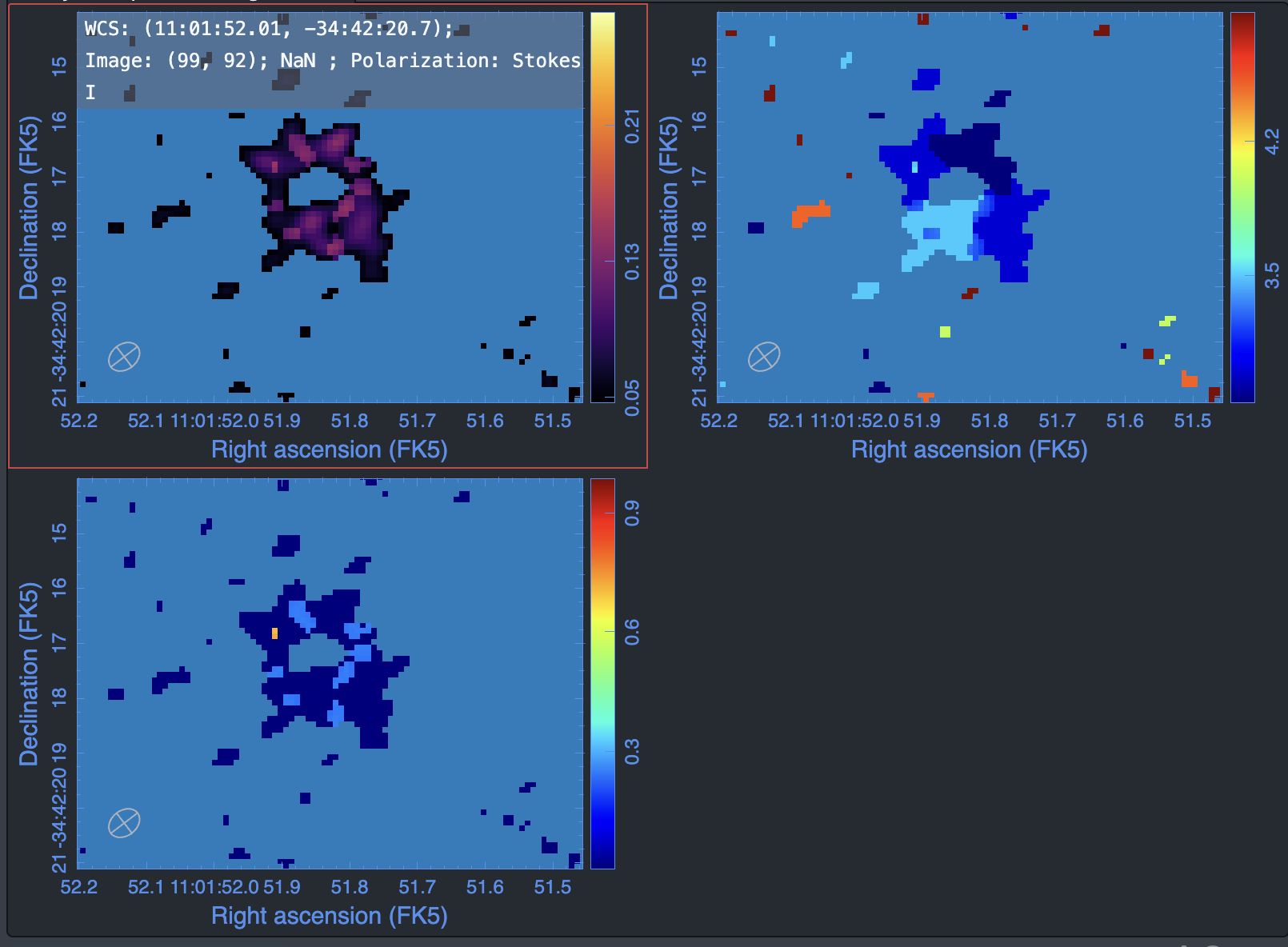
The final science product is the primary-beam-corrected cube:
twhya.final.cube.image.pbcor
Begin by measuring the RMS noise in several line-free channels and compare the values with those measured in the dirty cube. Next, inspect the cube in CARTA. Explore the data both spatially and spectrally:
- Play through the channels.
- Extract spectra from different regions.
- Identify the velocity range of emission.
- Examine the spatial distribution as a function of velocity.
These simple exploratory analyses already yield the first scientific insights from a spectral-line dataset.
Next, check the spectral line profile, extract spectra from different regions and also the integrated spectrum.
9. Exporting the Results
Although CASA stores images in its own native format, the FITS format remains the most widely used standard in astronomy.
Exporting the spectral cube and moment maps to FITS allows the data to be analysed using external software packages, archived and shared with collaborators.
In CASA
exportfits(
imagename='twhya.n2hp.image',
fitsimage='twhya.n2hp.fits',
velocity=True,
overwrite=True,
)
Similarly export the moment maps.
Other Related Pages
Introduction page.
EVN data on HI absorption against a compact radio source.
VLBA data on H₂O maser emission.