New generation imaging algorithms Hands-On with eht-imaging

Data and software required

Before simulating anything, we install/load ehtim and the standard libraries.

1. jet_model.txt — jet sky model in ehtim text format. Without this file the tutorial falls back to a point source.
2. ehtim 1.2.10 installed in your Python environment.

The files needed for this tutorial are bundled in the tar file below:

• ERIS26_new_imaging_algorithms.tar.gz

Alternatively, you can download and un-tar the data from the command line:

wget https://www.jb.man.ac.uk/ERIS26/data/ERIS26_new_imaging_algorithms.tar.gz
tar -zxvf ERIS26_new_imaging_algorithms.tar.gz

Important note on the Fourier engine (ttype): Throughout this tutorial we explicitly set ttype='fast' or 'direct' in every call to .observe() and to the Imager, avoiding any dependency on NFFT.

Table of contents

1. Array configuration: EVN vs. EVN+AVN
2. Sky model and the ideal observation
1. Observing parameters (C-band, 5 GHz)
2. Visualizing the uv-coverage
3. Realistic errors, self-calibration, and visibility corruption
1. Self-calibration
2. Visualizing the degradation: visibility amplitude vs. uv-distance
4. RML imaging: closures vs. raw visibilities
1. What is a "closure quantity"?
2. The imaging pipeline
3. Final visual comparison
4. Dirty beam, clean beam, and array resolution
5. Comparing regularizers: simple vs. tv vs. tv2
6. The effect of thermal-noise SNR
5. From this notebook to a real observation proposal
6. Extra: bring your own FITS source

1. Array configuration: EVN vs. EVN+AVN

← back to top

We define two antenna arrays:

• EVN: 11 real European/Asian stations, with their geocentric coordinates and their SEFD (System Equivalent Flux Density).
• EVN + AVN: the EVN combined with stations from the African VLBI Network (AVN). Adding African baselines substantially improves uv-coverage in the north-south direction.

# Load the arrays from the text files
array_evn = eh.array.load_txt('data/evn_array.txt')
array_comb = eh.array.load_txt('data/combined_array.txt')

print(f"EVN loaded: {len(array_evn.tarr)} stations")
print(f"EVN + AVN loaded: {len(array_comb.tarr)} stations")

2. Sky model and the ideal observation

← back to top

Our science case for this whole notebook is a realistic relativistic jet. We load it from a text-format model (jet_model.txt).

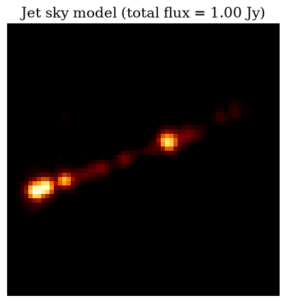
Figure 1: Jet sky model (total flux = 1.00 Jy) displayed with afmhot colormap.

2A. Observing parameters (C-band, 5 GHz)

We choose 5 GHz because it's a standard, realistic band for the EVN (C-band). We simulate the jet first under ideal conditions (no errors), our error-free reference for everything that follows.

# Simulating IDEAL observation (no errors)
obs_jet_ideal = im_jet.observe(
    array_comb, tint, tadv, tstart, tstop, bw,
    sgrscat=False, ampcal=True, phasecal=True, ttype='fast', add_th_noise=False
)
obs_jet_ideal.rf = nu
obs_jet_ideal.add_all(avg_time=avg_time)

2B. Visualizing the uv-coverage

To see what the AVN actually contributes, we also simulate the same ideal jet observation on EVN alone, purely for this comparison plot.

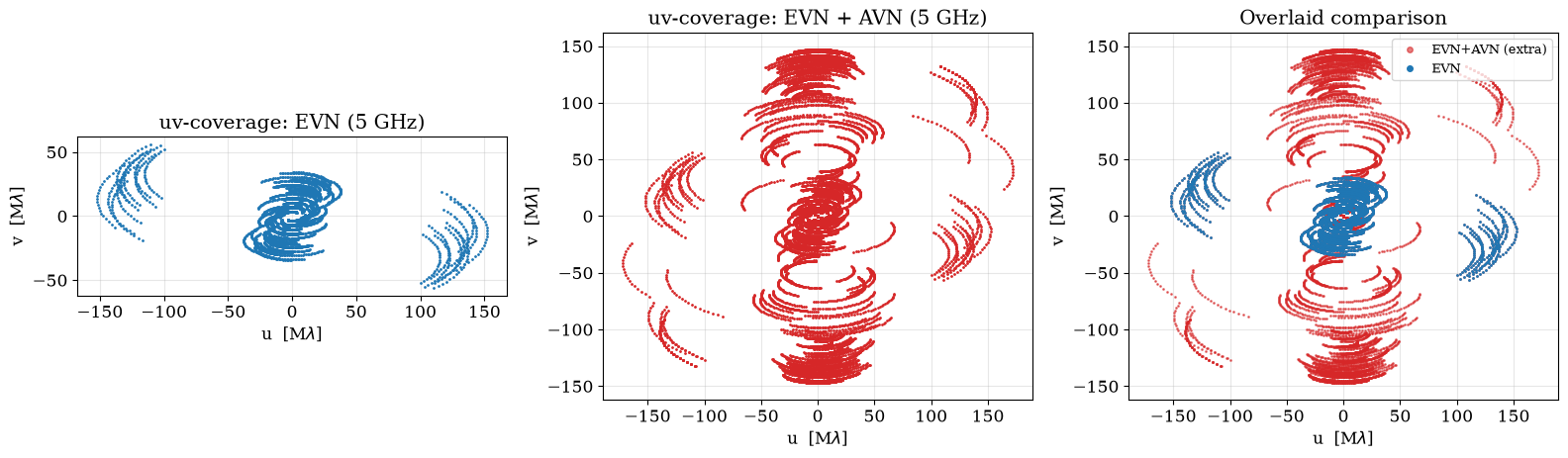
Figure 2: uv-coverage comparison between EVN (blue) and the combined EVN+AVN array (red). Notice how many NEW points the AVN contributes, especially in the north-south direction.

3. Realistic errors, self-calibration, and visibility corruption

← back to top

Real observations are affected by thermal noise, gain errors, phase drifts, etc. We inject these errors into our jet simulation and quantify the resulting degradation.

# CONTROLS TO EXPERIMENT WITH
gain_offset_val = 0.15   # Systematic amplitude gain error (e.g. 0.15 = 15%)
gainp_val       = 0.10   # Random amplitude gain error (per antenna)
elevation_min   = 10.0   # Minimum observing elevation [degrees]

obs_jet_err = im_jet.observe(
    array_comb, tint, tadv, tstart, tstop, bw,
    sgrscat=False, ttype='fast', elevmin=elevation_min,
    add_th_noise=True,                                            # thermal noise
    ampcal=False, gain_offset=gain_offset_val, gainp=gainp_val,   # amplitude errors
    phasecal=False                                                # phase errors
)

3A. Self-calibration

Self-calibration uses a model of the source to solve for the per-antenna gains that best explain the observed data, and applies them to correct the visibilities.

obs_jet_err.add_scans()   # essential for scan_solutions to group correctly
cal_jet = sc.self_cal(obs_jet_err, im_jet, ttype='fast', scan_solutions=True, processes=1)

3B. Visualizing the degradation: visibility amplitude vs. uv-distance

This is the single most-used diagnostic plot in the entire VLBI workflow. For a source with extended structure (like our jet), the amplitude falls off and oscillates in a pattern set by the source's morphology.

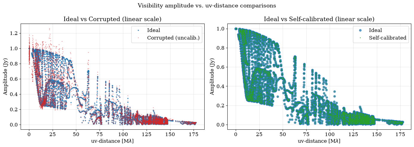
Figure 3: 'Ideal' shows the true source structure; 'Corrupted' shows the scatter introduced by errors; 'Self-calibrated' shows how much is recovered. The drop in amplitude at longer baselines represents resolved-out flux.

4. RML imaging: closures vs. raw visibilities

← back to top

4A. What is a "closure quantity"?

In real VLBI, every antenna has its own clock and atmosphere, introducing phase and amplitude errors. The visibility you actually measure on baseline $i$–$j$ is:

$$r_{ij} = \gamma_i \, \gamma_j^{*} \, V_{ij}$$

Closure quantities are special combinations of visibilities where every $\gamma_i$ term cancels out exactly. For example, the bispectrum ($V_{ijk} = V_{ij}V_{jk}V_{ki}$) and its argument, the closure phase ($\psi_{ijk} = \phi_{ij} + \phi_{jk} + \phi_{ki}$), are immune to per-antenna phase errors.

4B. The imaging pipeline

For an extended source, we progressively refine the image using a multi-round strategy:

• Round 1: Bispectrum (bs). Most robust to any kind of error.
• Round 2: amp + cphase. More spatial detail via closures.
• Round 3: vis (cal.). Switch to self-calibrated visibilities + closures for final absolute amplitude constraints.

4C. Final visual comparison

We compare the ideal reconstruction, the closure-based reconstruction on corrupted data, and the raw-visibility reconstruction on corrupted data using the NRMSE (Normalized Root-Mean-Square Error).

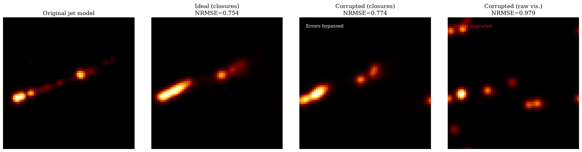
Figure 4: The closures-based reconstruction strongly outperforms the raw-visibility approach when systematic errors are present.

4D. Dirty beam, clean beam, and array resolution

The array's response to a point source (dirty beam) and the Gaussian fit to its main lobe (clean beam) tell us the true angular resolution limits of our observation.

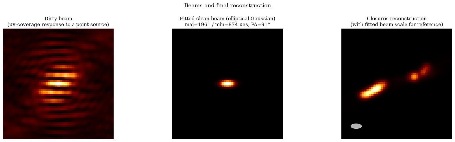
Figure 5: The Dirty Beam, Fitted Clean Beam, and the Final Reconstruction (with the clean beam overlaid) side-by-side.

4E. Comparing regularizers: simple vs. tv vs. tv2

Every RML round mixes a data term with a regularizer term. The choice between simple (diffuse), tv (sharp edges), or tv2 (softer edge preservation) dictates the morphology of the final image.

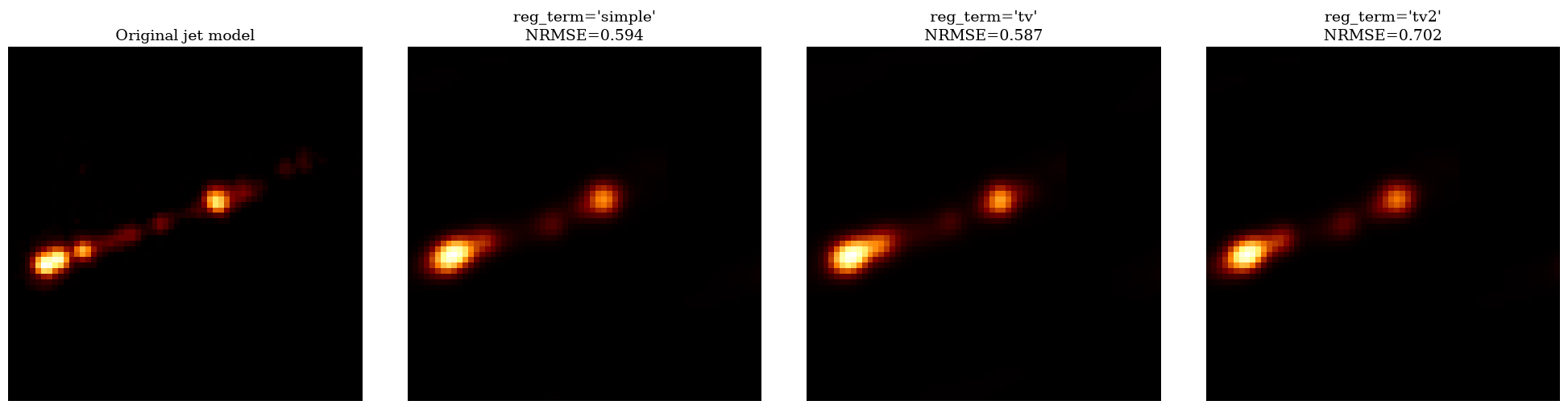
Figure 6: Reconstructions varying only the reg_term. Notice how 'tv' provides crisp boundaries ideal for jets.

4F. The effect of thermal-noise SNR

Even with perfect calibration, thermal noise limits image fidelity. Shorter integration times (`tint`) leave the reconstruction visibly noisier.

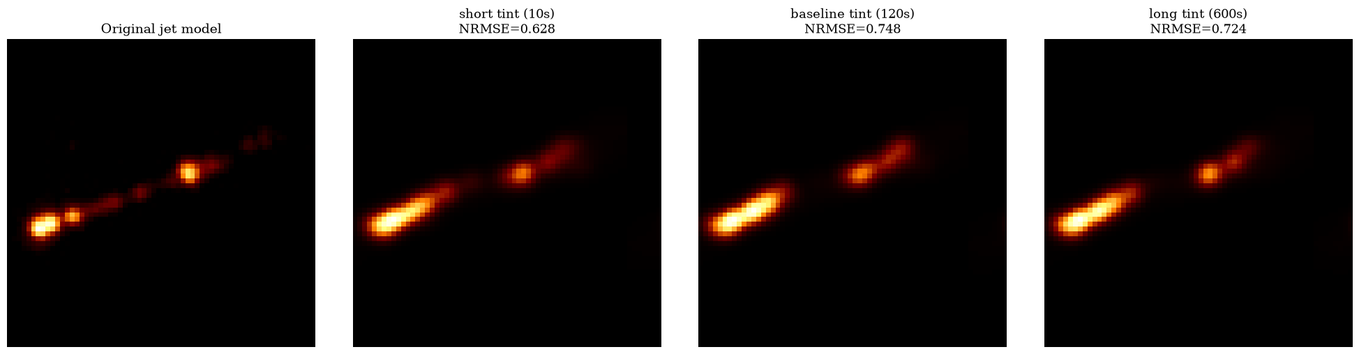
Figure 7: Impact of integration time (e.g., 4s vs 120s vs 3600s) purely due to thermal noise (no gain/phase errors).

5. From this notebook to a real observation proposal

← back to top

Everything you've produced here is a miniature feasibility study. A Time Allocation Committee will look for expected uv-coverage, expected sensitivity (NRMSE), and the simulated image reconstruction.

Export your outputs for papers or proposals using ehtim's built-in functions:

# Reconstructed image
im_rec_err_closure.save_fits('results/jet_reconstruction_closures.fits')
im_rec_err_closure.save_txt('results/jet_reconstruction_closures.txt')

# Visibility dataset (UVFITS for AIPS/CASA/Difmap)
obs_jet_err.save_uvfits('results/jet_observation_corrupted.uvfits')

# Save matplotlib figures
fig.savefig('results/jet_reconstruction_closures.png', dpi=200, bbox_inches='tight')

6. Extra: bring your own FITS source

← back to top

You can convert any 2D FITS image into an ehtim text model using the provided fits_to_ehtim_txt() function. The script will crop it to a square, normalize the flux, and run the entire simulation, self-calibration, and RML imaging pipeline automatically.