Advanced Tutorial - Polarisation
Goals of the tutorial
This tutorial is divided in two parts. First, we will produce and explore different sets of simulated full-polarization visibilities, in order to learn to recognize the different kinds of polarization signals (i.e., source-intrinsic versus instrumental). Then, we will work on a set of real VLBI full-polarization observations, to calibrate the instrumental effects, deconvolve polarized images and perform a basic analysis of the results.
Getting the software and data
The tutorial makes use of the CASA-based software called $\texttt{casa-poltools}$, which can be downloaded from:
CASA-poltools (GitHub 2026A Release).
Untar the contents of $\texttt{casa-poltools}$ in any directory of your choice. Then, compile it using the Python3 binary that comes with CASA. You just have to open a terminal, go to the $\texttt{casa-poltools}$ directory (that you have just created) and run the command:
PATH/TO/YOUR/CASA/bin/python3 setup.py build_ext --inplace
If something fails, you probably need the Python headers (in Ubuntu/Debian, you can install them with $\texttt{sudo apt install python3-dev}$) or some library that should be easily installed.
Once the code is compiled, you have to update the file $\texttt{.bashrc}$ (located in your $\texttt{\$HOME}$ directory) and add the line:
export PYTHONPATH=${PYTHONPATH}:/FULL/PATH/TO/CASA-POLTOOLS/DIRECTORY
Beware of not adding spaces in that line! And that's it! Now, you can run the $\texttt{casa-poltools}$ by just starting CASA and loading the modules by writing these lines in the CASA prompt:
from task_polsimulate import polsimulate
from task_polsolve import polsolve
- To run all the steps in the tutorial, you have to download the datasets and scripts from this link:
wget https://www.jb.man.ac.uk/ERIS26/data/ERIS26_polarisation_tutorial.tar.gz - Un-tar the download using
tar -zxvf ERIS26_Data_polarisation.tar.gz
You should find the following files in your folder:
running_polsimulate.py- Script to generate (and process) all the simulations of the first part of the tutorial.running_polsolve.py- Script to estimate (and apply) the instrumental polarization in the simulations used in this tutorial.EHT.cfg- Array configuration file to simulate the Event Horizon Telescope (in its 2017 campaign).EHT_M87_11Apr2017.listobs- List of scans corresponding to the M87* EHT observations on April 11, 2017. This file will be used by $\texttt{polsimulate}$, to generate synthetic EHT data reproducing the same UV coverage as the real observations.EHT_11Apr2017_M87.ms- Measurement set containg the Event Horizon Telescope (EHT) observations of M87* taken on April 11, 2017, already self-calibrated and ready for imaging and D-term calibration.EHT_ERIS26_polsolve.py- script for the second part of the tutorial (M87* data).VLBA_BG251A_7mm.ms- Multi-source VLBA observations at 43GHz, taken on year 2017, after fringe-fitting, amplitude calibration, and hybrid imaging (i.e., self-calibration). The data are ready for the calibration of the instrumental polarization.VLBA_ERIS26_polsolve.py- script for the second part of the tutorial (VLBA data).
The tutorial scripts don't have blanks, as most parameter settings are unambiguous. There are, though, some steps where you will have to figure out a few other things, as well as optional extra activities suggested across the tutorial, if you have time.
You can find a complete guide to display polarization information in CARTA here: Displaying polarization in CARTA
Table of contents
Part 0. Software and Scripts
Part I. Simulations
- Unpolarized point source (no Dterms).
- Unpolarized point source (with Dterms).
- Polarized point source (no Dterms).
- Polarized point source (with Dterms).
- Double polarized source (no Dterms).
- Double polarized source (with Dterms).
- Double polarized source (with cross-delay).
Part II. Real Data
Additional Material
- Unpolarized point source (no Dterms).
- Unpolarized point source (with Dterms).
- Polarized point source (no Dterms).
- Polarized point source (with Dterms).
- Double polarized source (no Dterms).
- Double polarized source (with Dterms).
- Double polarized source (with cross-delay).
Part II. Real Data
Additional Material
Part 0: Software and Scripts
Description of PolSimulate
For the first part of the tutorial, we will make use of the $\texttt{casa-poltools}$ program $\texttt{polsimulate}$, as well as $\texttt{plotms}$, $\texttt{iclean/tclean}$, $\texttt{polcal}$ and $\texttt{CARTA}$. We will also use some other auxiliary functions provided in $\texttt{casa-poltools}$, like $\texttt{plotPolImage}$ and $\texttt{plotPolTraces}$. Here we describe the main arguments of $\texttt{polsimulate}$, which will allow us to generate realistic full-polarization synthetic datasets under different instrumental conditions:
Parameters related to the data and the instrument:
- $\texttt{vis}$: Name of the measurement set to be populated with the synthetic data.
- $\texttt{array_configuration}$: ASCII file containing the names, coordinates and mount types of the antennas to be simulated. We will use the file $\texttt{EHT.cfg}$, provided for the tutorial, although you have other example files in the $\texttt{casa-poltools/TESTS}$ directory.
- $\texttt{plot_elevs}$: If True, the program makes a plot of antenna elevations versus time.
- $\texttt{model_Dt_0}$: List of instrumental polarization (D-terms) for the first polarization channel (i.e., RCP, if circular polarization is used) of all antennas. For the most simple simulations (the ones that we will be doing here), this is just a list of complex numbers (i.e., the D-terms), one per antenna.
- $\texttt{model_Dt_1}$: Instrumental polarization (D-terms) for the second polarization (LCP) of all antennas (one complex number per antenna).
- $\texttt{Kcross}$: Cross-polarization delay of the reference antenna (in seconds). RCP (or X) is taken as reference.
- $\texttt{feed}$: The polarization feed to simulate (in our case, this will always be $\texttt{"circular"}$).
- $\texttt{LO}$: Center observing frequency (in Hz).
- $\texttt{BBs}$: List of baseband frequencies (in Hz), one per spectral window to be simulated. The actual frequencies of the spectral windows are $\texttt{LO}$ + $\texttt{BBs}$.
- $\texttt{spw_width}$ and $\texttt{nchan}$: Width (in Hz) and number of channels of the spectral windows. The same values are used for all of them.
- $\texttt{nscan}$: Number of scans to simulate. If the path to a $\texttt{listobs}$ file is given instead, the observing times of the scans will be taken from the $\texttt{listobs}$ contents.
- $\texttt{visib_time}$: Integration time used at the correlator (in s).
- $\texttt{apply_parang}$: Whether to apply the parallactic-angle correction (in principle, this should be set to True).
- $\texttt{corrupt}$: Whether to add thermal noise to the visibilities (the default values for System Temperatures, gains, atmospheric opacity, etc., based on the CASA simulator, should be fine).
Parameters related to the source:
The source structure (in full polarization) can be given either from a CASA (model) image or as a set of polarized point sources (which is the option that we will use here). In this case, the parameters for the point sources are:
- $\texttt{phase_center}$: The sky coordinates of the phase center, in standard format. For example:
$\texttt{"J2000 17h45m40.4230 -29d00m28.0400"}$. - $\texttt{RA_offset}$: List of offsets in right ascension (in arcsec), with respect to the $\texttt{phase_center}$. One value per point source to be simulated.
- $\texttt{Dec_offset}$: List of offsets in declination (in arcsec). One value per point source.
- $\texttt{I}$: List of flux densities (in Jy) for the point sources (in consistent order with the previous lists).
- $\texttt{Q_frac}$, $\texttt{U_frac}$ and $\texttt{V_frac}$: Lists of fractional Stokes Q, U and V (respectively) for each of the point sources to simulate.
- $\texttt{RM}$ and $\texttt{spec_index}$: Lists of Rotation Measures and spectral indices (we will not use any of these).
For example, setting $\texttt{RAoffset=[0.0]}$; $\texttt{Decoffset=[0.0]}$; $\texttt{I=[1.0]}$; and $\texttt{Q_frac=U_frac=V_frac=[0.0]}$ will simulate a single unpolarized point source at the phase center.
Simulation script:
The script running_polsimulate.py runs $\texttt{polsimulate}$ programatically and can be configured by setting a few parameters at its header. The most important one is $\texttt{CASE}$, an integer that sets the different sources (and D-terms) depending on its value. In particular, the cases included in the script are:
- Unpolarized point source with no instrumental polarization (the simplest case).
- Unpolarized point source with instrumental polarization (to learn how to identify D-term effects).
- Polarized point source without instrumental polarization (to learn how to identify source-intrinsic polarization).
- Polarized point source with instrumental polarization (a more realistic scenario).
- Polarized double source without instrumental polarization (closure traces will be interesting here).
- Polarized double source with instrumental polarization (how will closure traces compare with the case above?).
- A different polarized double source (how will closure traces compare with the cases above?).
- Polarized point source with D-terms and cross-polarization delay (we will try to calibrate both quantities).
Another relevant script parameter is $\texttt{DtermAmp}$, which sets the amount of instrumental polarization to simulate. The Dterms are set from a complex random Gaussian distribution, centered at zero with a width equal to $\texttt{DtermAmp}$. It may be a good idea to repeat some of the script cases by increasing $\texttt{DtermAmp}$, so you can see how a more important instrumental polarization may affect the visibilities.
Regarding the radiotelescopes, we will use the array configuration of the Event Horizon Telescope in its campaign of year 2017. The antenna coordinates, sizes, and mount types are given in the file EHT.cfg. The exact observing times used in our simulations will be extracted from those of the real EHT observations of M87* on April 11, 2017. This information will be provided to $\texttt{polsimulate}$ via the file EHT_M87_11Apr2017.listobs
Description of PolSolve
For the second part of the tutorial (and some exercises of the first part), we will make use of $\texttt{polsolve}$, a program that estimates the instrumental polarization and applies it to the data, allowing us to deconvolve full-polarization images. The most important parameters of $\texttt{polsolve}$ (at least, the ones that we will use here) are:
- $\texttt{vis}$: Name of the measurement set to calibrate in polarization.
- $\texttt{caltable}$: Name of the output Dterms calibration table.
- $\texttt{field}$: Name (or ID) of the source(s) to be used as calibrator(s).
- $\texttt{target_field}$: Name (or ID) of the source(s) to be used as the target(s) (can be equal to $\texttt{field}$). The program will apply the estimated D-terms to the $\texttt{corrected}$ data column of the fields given here.
- $\texttt{DR}$ and $\texttt{DL}$: Lists (or dictionaries) of a-priori D-terms for RCP and LCP, respectively (default is zero). One value (complex number) per antenna. If a list is used, we assume the same order than that of the $\texttt{ANTENNA}$ table. If a dictionary is given, the keywords will be the antenna names (codes).
- $\texttt{DRSolve}$ and $\texttt{DLSolve}$: Lists (or dictionaries) of booleans (one value per antenna). If True, the D-term of that antenna will be fitted; if False, it will be fixed to its a-priori value. Default is True for every antenna.
- $\texttt{CLEAN_models}$: Setting it to $\texttt{"model_column"}$ will use the full-polarization model stored in the model column of the measurement set (populated, for instance, by $\texttt{iclean}$ or $\texttt{tclean}$) as the source model. Otherwise, we can define the source model as a set of point sources, in a similar way as it is done in $\texttt{polsimulate}$ (although, in this case, the polarization properties of each point source are given in the lists called $\texttt{frac_pol}$ and $\texttt{EVPA}$). In this tutorial, we will (almost) always set it to $\texttt{"model_column"}$.
- $\texttt{plot_parang}$ and $\texttt{plot_residuals}$: It's good to set these to True, so we can check the time evolution of the parallactic angles of the antennas and the post-fit cross-polarization visibility residuals in phasor space.
Calibration script:
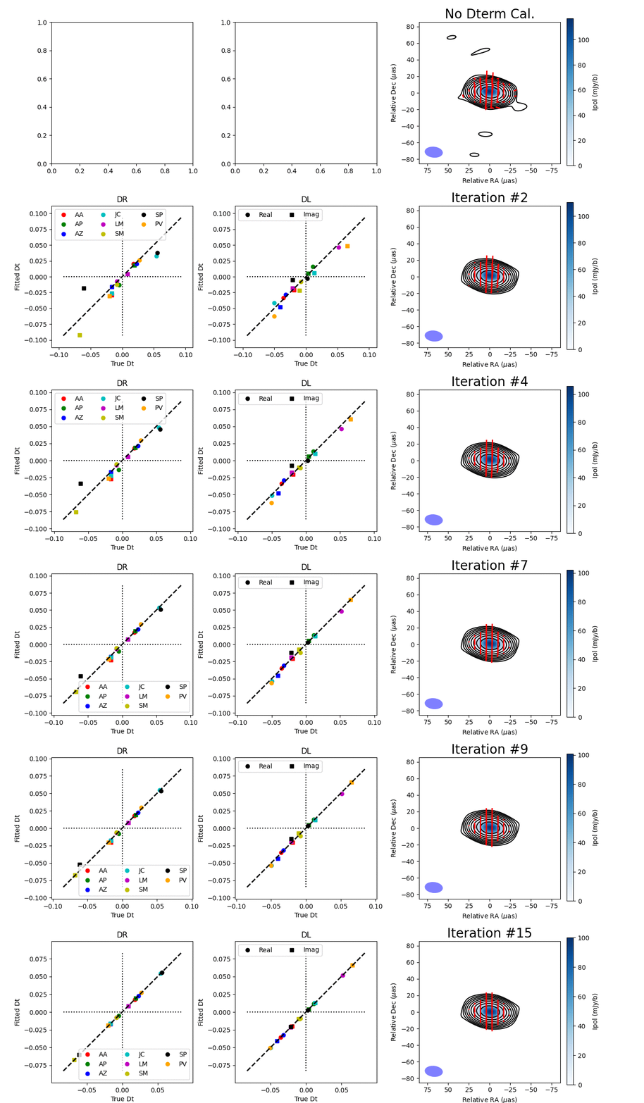
The script running_polsolve.py estimates the D-terms of a measurement set using $\texttt{polsolve}$. The strategy followed is similar to a self-calibration, but in polarization. The idea is to iterate the following steps:
- Build a full-polarization image of the $\texttt{field}$ source(s) (use $\texttt{iclean}$ first, to define a mask, and $\texttt{tclean}$ later, in automatic mode using that mask). The $\texttt{model}$ column of the measurement set will be populated with the visibility matrices computed from the CLEAN model.
- Estimate the antenna D-terms with $\texttt{polsolve}$, by nimimizing the residuals between the $\texttt{data}$ and the $\texttt{model}$ columns.
- Apply the estimated D-terms to the $\texttt{target_field}$ (which we make equal to $\texttt{field}$), by populating the $\texttt{corrected}$ column. This is done automatically by $\texttt{polsolve}$.
- Go back to step 0, but using the $\texttt{corrected}$ column for the full-polarization deconvolution.
- For simulated data: Correlation plots between the estimated D-terms and the ground-truth D-term values used in $\texttt{polsimulate}$.
- For real data: The estimated D-terms.
Once the D-terms have converged (after a few iterations of the steps described above), the script applies them one last time, to generate the final $\texttt{corrected}$ column. Then, a final run of $\texttt{tclean}$ generates the full-polarization image of $\texttt{target_field}$ (i.e., $\texttt{field}$).
The parameters to set up the script are given in its header. In particular:
- $\texttt{vis}$: The measurement set to calibrate.
- $\texttt{field}$: The name(s) or ID of the source(s) to be used as calibrator(s). If the measurement set only contains one source, it can be set to just $\texttt{"0"}$.
- $\texttt{polNiter}$: Number of $\texttt{tclean}$-$\texttt{polsolve}$ iterations to estimate the D-terms.
- $\texttt{imagename}$, $\texttt{weighting}$, $\texttt{niter}$, $\texttt{gain}$, $\texttt{cell}$, and $\texttt{imsize}$: Homologous to the $\texttt{iclean}$ and $\texttt{tclean}$ parameters to be used in the iterations.
- $\texttt{ground_truth}$: If we are using a simulation, this should be the name of the binary table where the ground-truth D-terms have been stored (i.e., the file that ends with "$\texttt{*.true-dterms}$").
Part I: Simulations
CASE=0. Unpolarized point source (no D-terms)
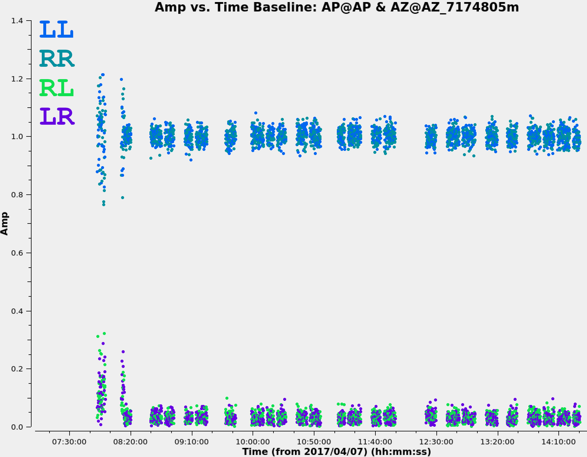
We will set $\texttt{CASE = 0}$ in the simulation script, running_polsimulate.py, and run it from CASA. If the installation of $\texttt{casa-poltools}$ was OK, it should soon generate a measurement set called POLSIM_CASE_0.ms, corresponding to an unpolarized point source located in the same coordinates as SgrA* (i.e., we have replaced SgrA* by a synthetic point source), and observed with the EHT in its exact configuration of April 7, 2017.
Explore the visibilities with $\texttt{plotms}$. The interesting quantities are amplitude (and phase) vs. time (and UV-distance) for all four correlation products, $\texttt{RR}$, $\texttt{RL}$, $\texttt{LR}$, and $\texttt{LL}$.
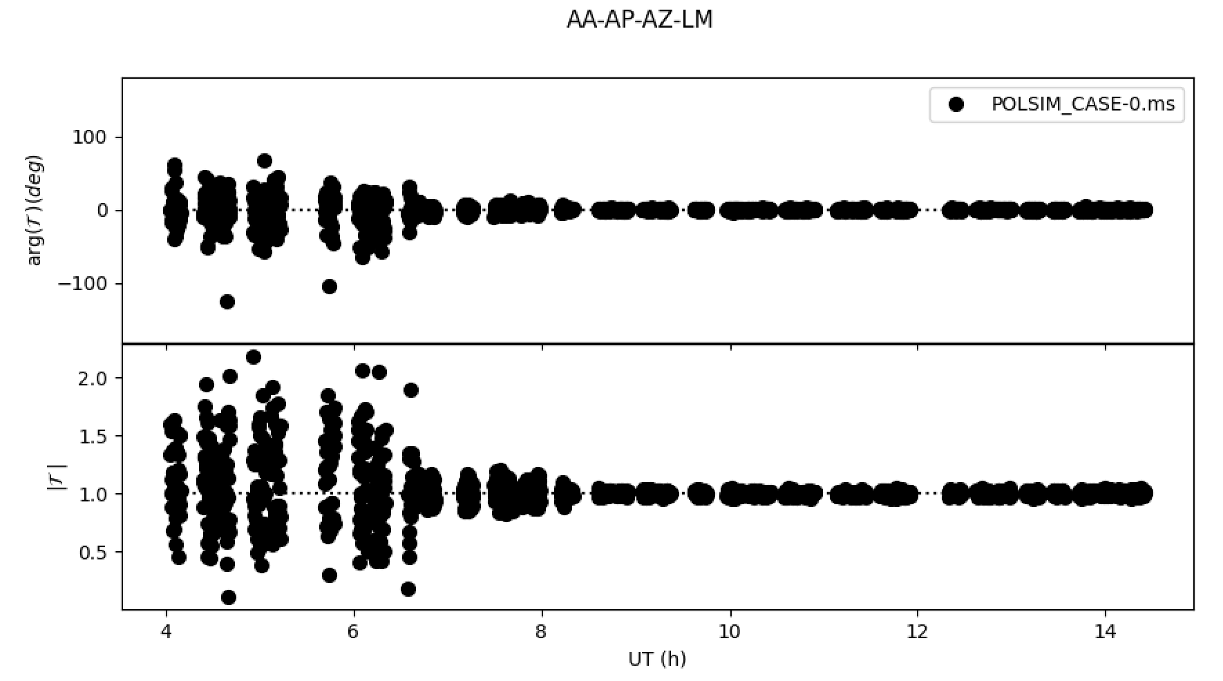
EXERCISE: Use the helper function $\texttt{plotPolTraces}$ to plot the closure traces for the antenna quadruplet ALMA-APEX-LMT-SMT (AA-AP-LM-AZ). Comment on the results. This function is called by running the lines:
from poltools_helper import plotPolTraces
plotPolTraces(vis=["POLSIM_CASE-0.ms"],antennas=["AA","AP","LM","AZ"])
CASE=1. Unpolarized point source (with D-terms)
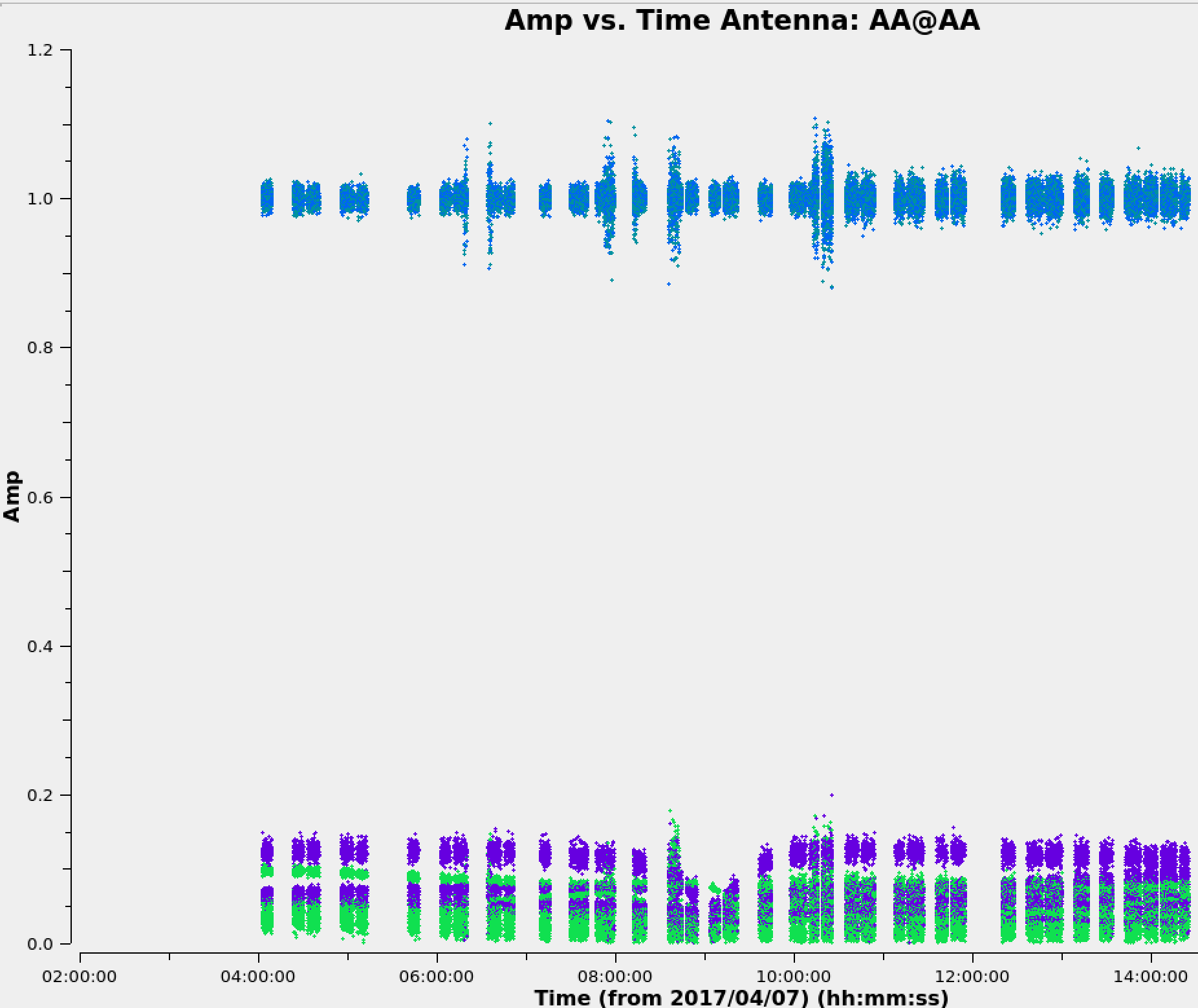
By setting $\texttt{CASE = 1}$ in the simulation script, we will generate the measurement set POLSIM_CASE_1.ms, corresponding to a source with no polarization, but observed with an imperfect interferometer (i.e., affected by instrumental polarization).
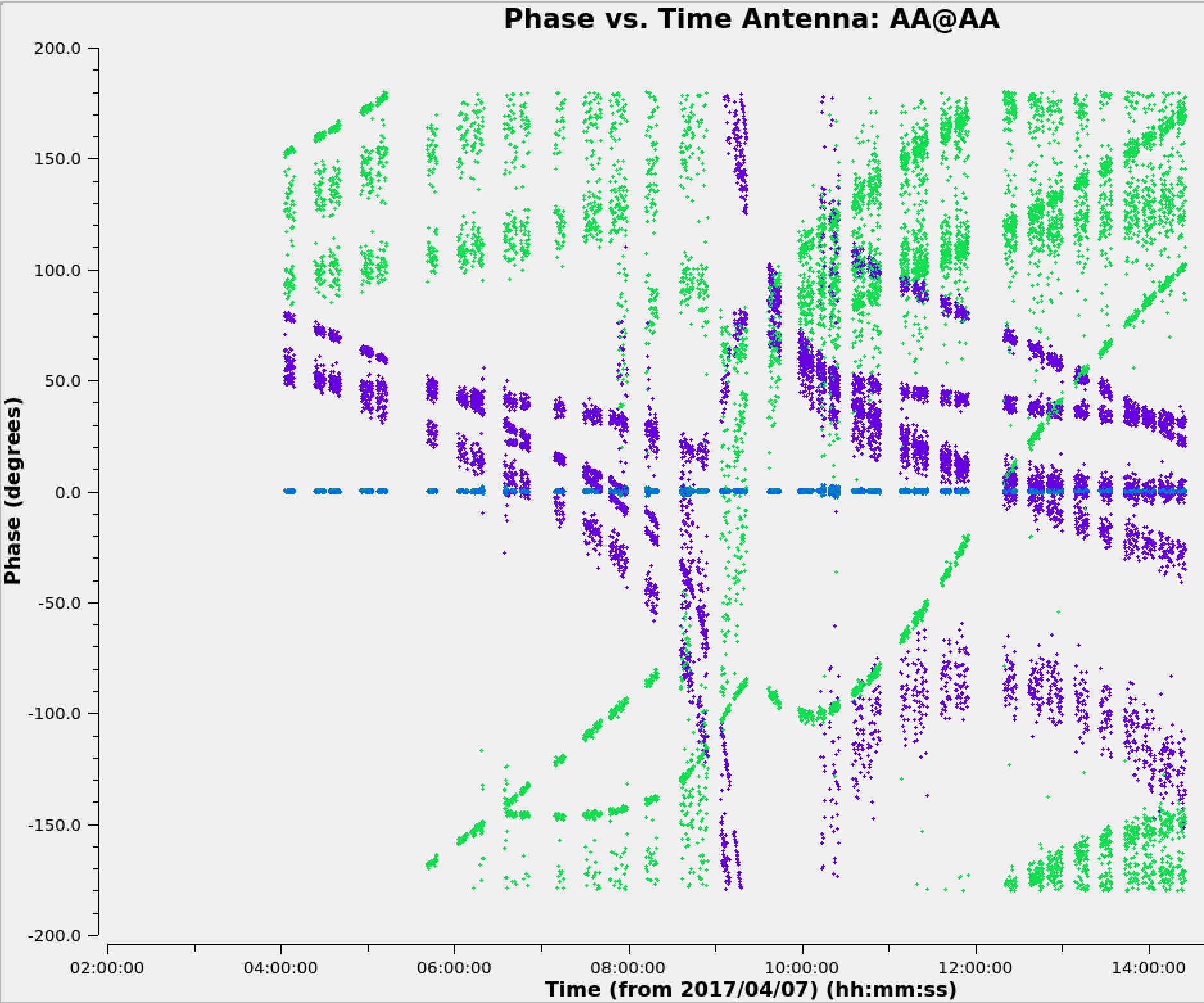
QUESTION: Explore the parallel-hand visibilities, $\texttt{RR}$ and $\texttt{LL}$ (in amplitude and phase) versus time and compare them to those of the previous case (i.e., unpolarized source with no instrumental polarization). Comment on the results.
QUESTION 2: Now, repeat the previous comparison, but with the cross-hand visibilities, $\texttt{RL}$ and $\texttt{LR}$. Do you see any qualitative difference with respect to the parallel-hand visibilities? Why?
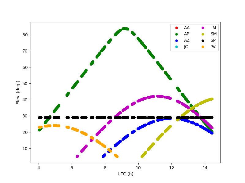
QUESTION 3: You may see rapid changes (especially in the visibility phases) for some baselines at some particular time ranges. What do you think is happening? Plotting the antenna elevations versus time (i.e., $\texttt{plot_elevs=True}$) may be helpful.
EXERCISE: Use the function $\texttt{plotPolTraces}$ to plot the closure traces for the antenna quadruplet ALMA-APEX-LMT-SMT (AA-AP-LM-AZ), as you did in the previous case. How does the new figure compare to that of $\texttt{CASE=0}$? Comment on the results.
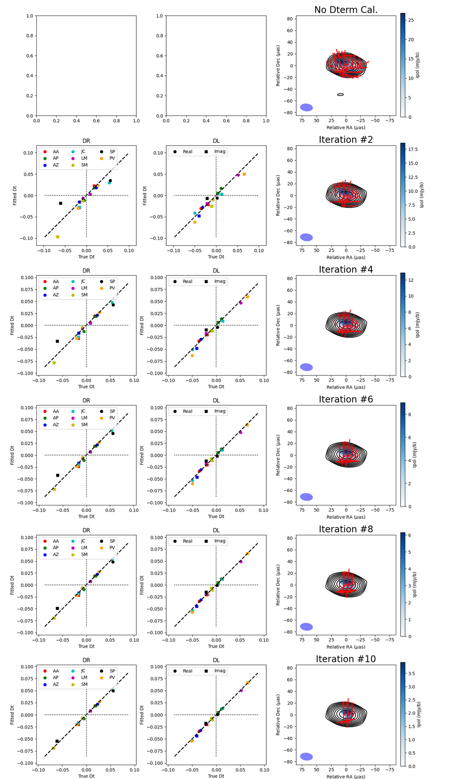
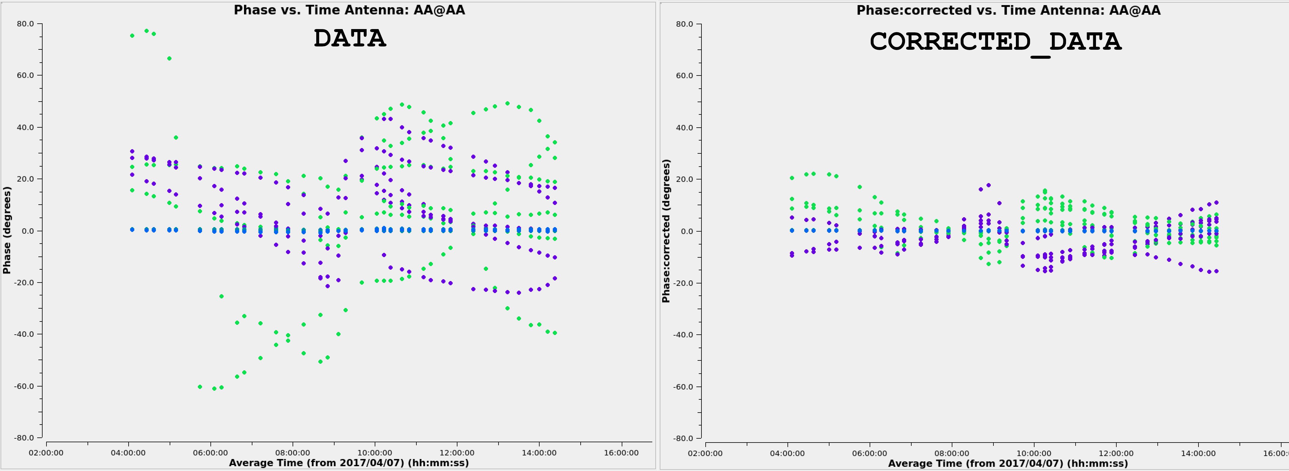
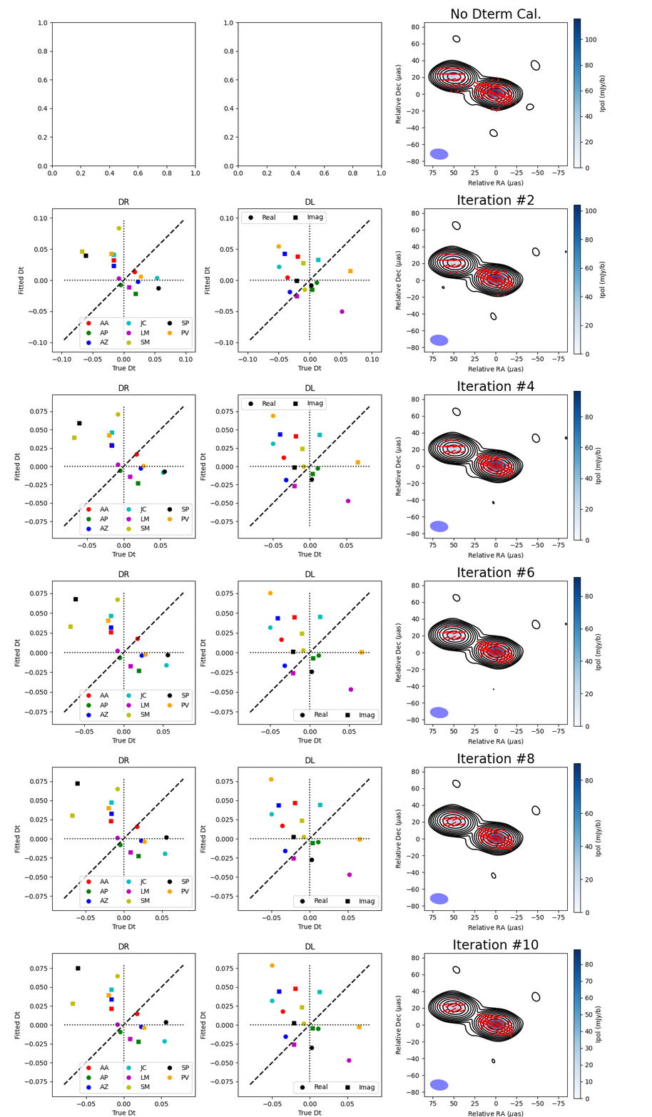
EXERCISE 2: Use the script $\texttt{running_polsolve.py}$ to solve for the D-terms (just a handful of iterations should suffice). Check the correlation plots between true D-terms and estimated D-terms and discuss on the results. Now, use $\texttt{plotms}$ to plot the cross-hand visibilities of the $\texttt{CORRECTED_DATA}$ column and comment on the results.
CASE=2. Polarized point source (no D-terms)
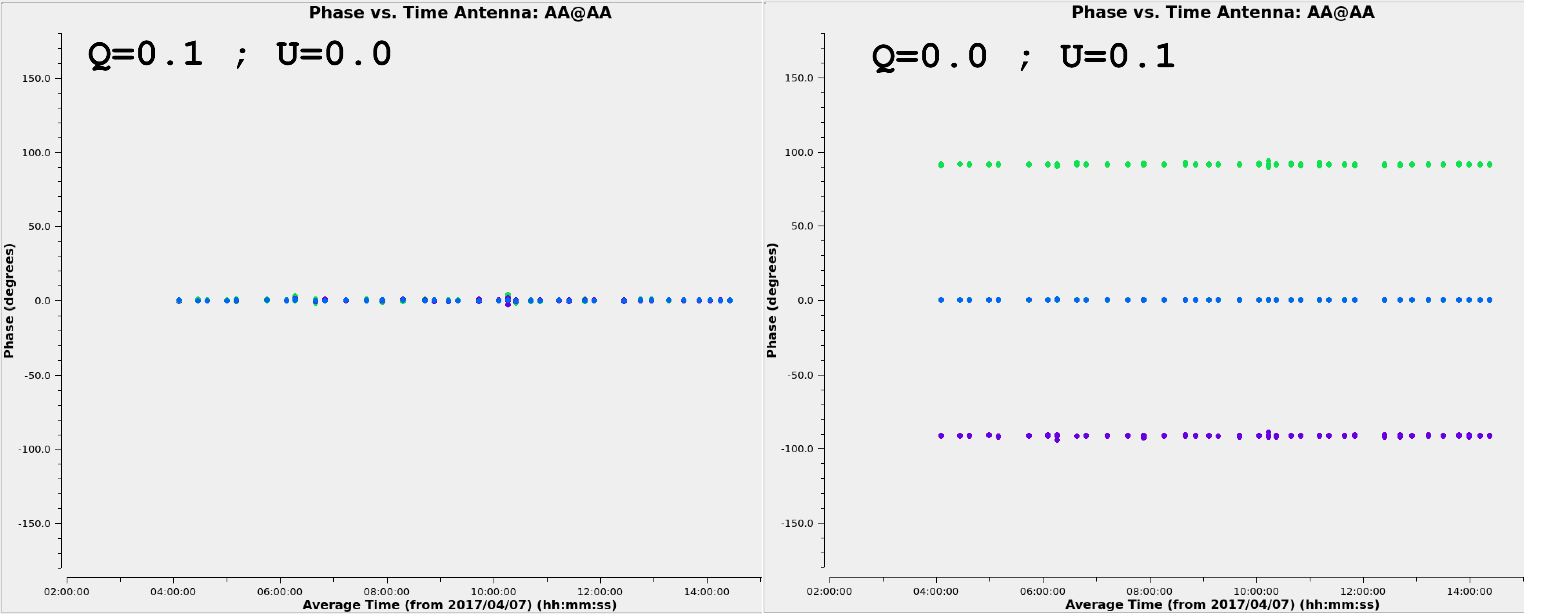
By setting $\texttt{CASE = 2}$ in the simulation script, we will generate the measurement set POLSIM_CASE_2.ms, corresponding to a source with Stokes parameters $\texttt{I=1.0}$Jy, $\texttt{Q=0.1/I}$, $\texttt{U=0.0/I}$, $\texttt{V=0.0/I}$. Explore, again, the visibilities with $\texttt{plotms}$, as you did with the previous cases.
EXERCISE: What are the phases of $\texttt{RL}$ and $\texttt{LR}$? Re-generate the measurement set with $\texttt{Q=0.0/I}$, $\texttt{U=0.1/I}$ (i.e., exchanging $\texttt{U}$ and $\texttt{Q}$). What happens to the phases of $\texttt{RL}$ and $\texttt{LR}$? How does this relate to the Visibility Matrix in the Measurement Equation? Do you think that, once the data are fully calibrated, the RL phases may always be the opposite of the LR phases? Why?
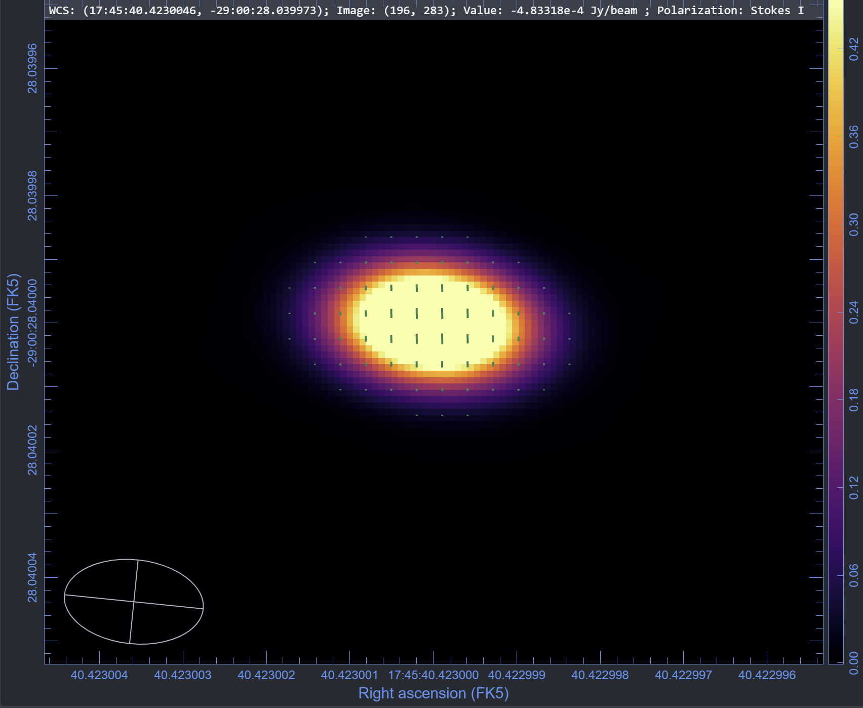
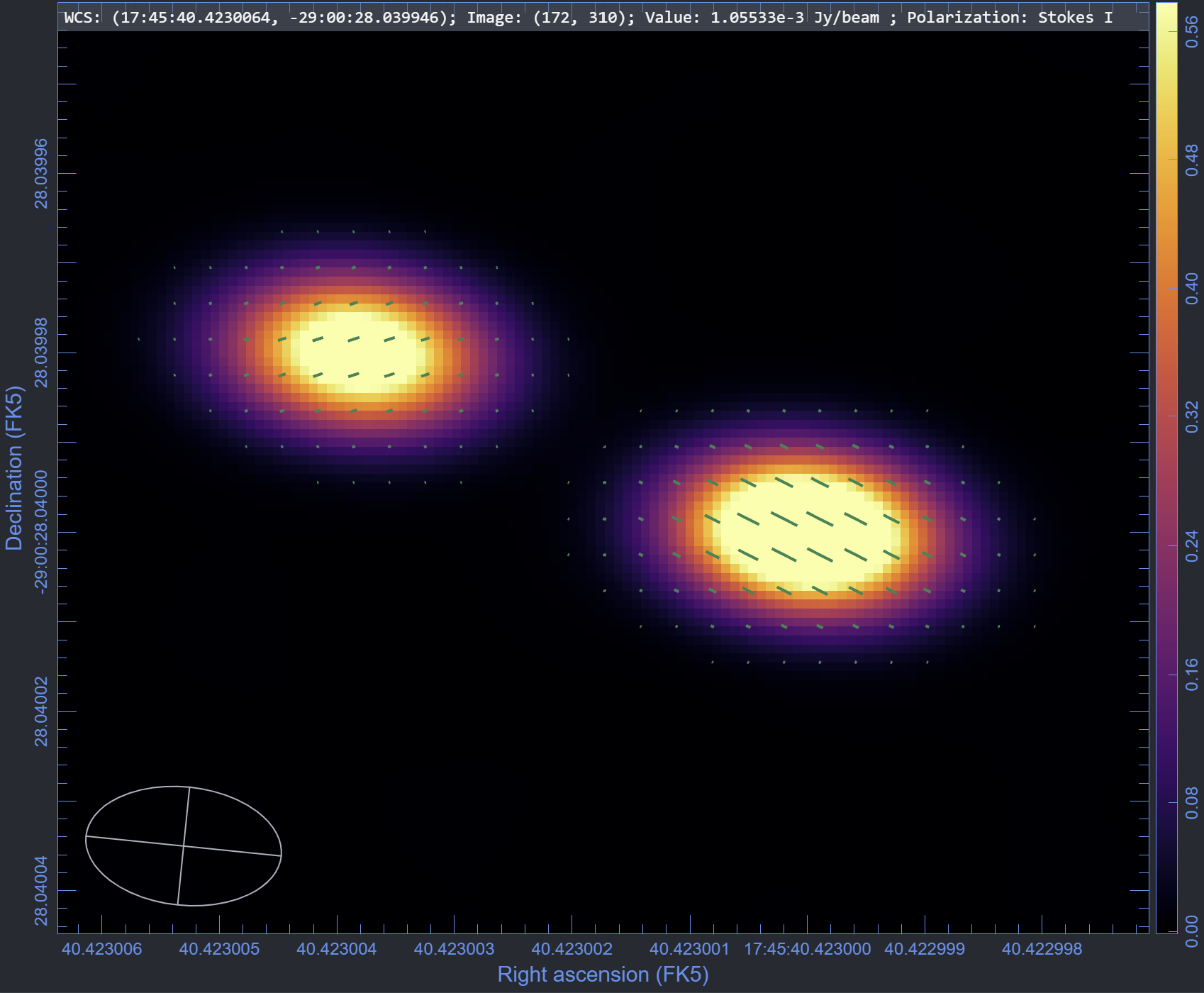
EXERCISE 2: Run $\texttt{iclean}$ on the last measurement set, using $\texttt{stokes="IQUV"}$. You should set the weighting to $\texttt{uniform}$ and the pixel size to about $\texttt{0.001 mas}$. The CASA image will have four polarization channels (I, Q, U, and V). Then, plot the image in $\texttt{CARTA}$, with raster (and/or contours) reflecting total intensity and lines (on top of the raster) to show the EVPA and intensity of the polarization.
- Alternatively to the use of $\texttt{CARTA}$, the image of polarized intensity can be generated in $\texttt{immath}$, using $\texttt{mode="poli"}$ and setting $\texttt{sigma}$ to the noise level (rms) of the image.
- The image with the EVPA information can also be generated in $\texttt{immath}$, using $\texttt{mode="pola"}$ and setting $\texttt{polithresh}$ to 3-5 times the rms.
- Another alternative is to use $\texttt{casa-poltools}$ to generate the polarized image. Just run, for instance:
(you have a description of all the $\texttt{plotPolImage}$ parameters by doing: $\texttt{help(plotPolImage}$).from poltools_helper import plotPolImage plotPolImage(img='CASE-2_IMG.image', mSigmaCut=2.0, SigmaCut=2.0, dPol=7, lPol=0.1, zoom=3)
EXERCISE: Plot the closure traces for the quadruplet ALMA-APEX-LMT-SMT and compare them to those from the previous cases. Comment on the results.
CASE=3. Polarized point source (with D-terms)
By setting $\texttt{CASE = 3}$ in the simulation script, we will generate the measurement set POLSIM_CASE_3.ms, corresponding to a source with the same Stokes parameters as in $\texttt{CASE = 2}$, but with instrumental polarization added to the signal. Explore the visibilities with $\texttt{plotms}$ and compare the results to those in the previous cases.
QUESTIONS: How do the cross-polarization amplitudes and phases (vs. time) compare to those of $\texttt{CASE = 1}$? And those of $\texttt{CASE = 2}$? How could we disentangle the source-instrinsic polarization from the instrumental signal?
EXERCISE: Run $\texttt{iclean}$ on this measurement set without performing any D-term calibration, and plot the full-polarization image in $\texttt{CARTA}$. How does the noise level in the polarization intensity compare to that of $\texttt{CASE = 2}$? Is the peak value of polarization intensity (or the EVPA at the peak) much affected by the D-terms?
OPTIONAL EXTRA EXERCISE 2: Repeat the previous exercise, but re-generating the measurement set with much larger (say, 3 times larger) D-terms. This can be done by increasing the value of $\texttt{DtermAmp}$. Compare results.
EXERCISE 3: Plot the closure traces for the quadruplet ALMA-APEX-LMT-SMT and compare them to those from the previous cases. Comment on the results.
EXERCISE 4: Use the script $\texttt{running_polsolve.py}$ to solve for the D-terms. Use $\texttt{plotms}$ to plot the cross-hand visibilities of the $\texttt{CORRECTED_DATA}$ column. How do these visibilities compare to those of $\texttt{CASE=2}$ (i.e., without D-term contamination)?
Solving for the source polarization simultaneously
The procedure followed in $\texttt{running_polsolve.py}$ is qualitatively similar to hybrid mapping (i.e., the process of self-calibration coupled to deconvolution). In this process, the source model is kept fixed when the D-terms are estimated.
However, if the source structure is very simple (e.g., a point source) it is possible to estimate the source polarization model and the D-terms simultaneously, hence optimizing convergence.
$\texttt{polsolve}$ can fit the polarization of calibrators with relatively resolved brightness distributions, modelling them as a set of point (delta) components. Each component (or subset of components) can be assigned one fractional polarization and EVPA, which will be fitted together with the antenna D-terms. Let's redo the calibration of
In this case, $\texttt{CLEAN_models}$ is a list of one Stokes I flux density (i.e., there is only one point source), $\texttt{frac_pol}$ is the (list of) a-priori fractional polarization of the point source and $\texttt{EVPA}$ is its a-priori polarization angle. Regarding $\texttt{PolSolve}$, it is a list of booleans (one per point source) that tells $\texttt{polsolve}$ whether the polarization of the point sources has to be fitted or kept fixed (True means to be fitted).polsolve(vis='POLSIM_CASE-3.ms', caltable='CASE-3_With-Source-Fitting.dterms', CLEAN_models=[1.0], frac_pol=[0.0], EVPA=[0.0], PolSolve=[True])
Once you have run the code, take a look at the text printed by $\texttt{polsolve}$ in the terminal. You will see an estimate of the polarization state of the point source, as well as the D-terms. You can compare the numbers by eye to those printed by $\texttt{polsimulate}$ when you generated the measurement set. However, it is a much better idea to generate correlation plots. To do this, just execute these lines:
from poltools_helper import compareDterms
compareDterms(dt1='POLSIM_CASE-3.true-dterms',dt2='CASE-3_With-Source-Fitting.dterms')
This function will generate a plot of the correlation between the true D-terms and the ones just estimated by $\texttt{polsolve}$ (the table is called $\texttt{CASE-3_With-Source-Fitting.dterms}$).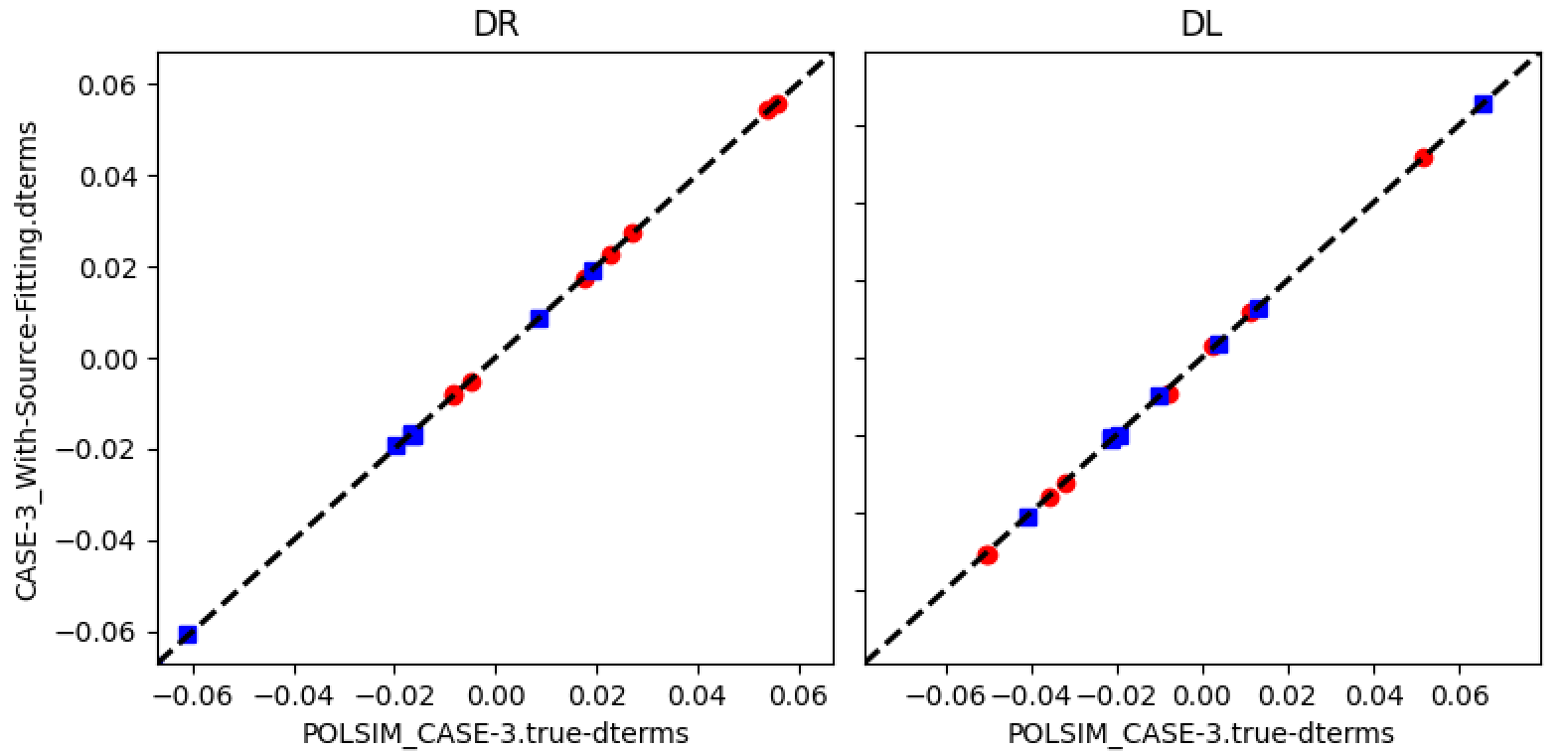
Using CASA's $\texttt{polcal}$ task
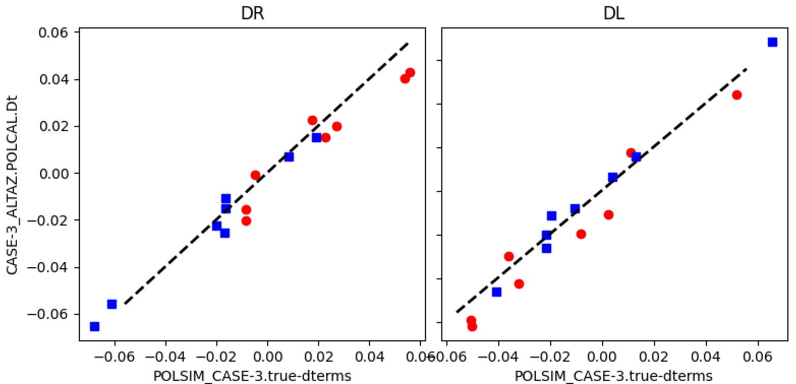
CASA has a built-in task called $\texttt{polcal}$, able to estimate the instrumental polarization (D-terms) and their possible frequency dependence. As in the fitting above, $\texttt{polcal}$ can also fit for the source polarization at the same time as the D-terms. Even though the use of this task is very simple, it has some limitations. Mainly:
- The calibrator is assumed to be point-like. This limitation is especially important for VLBI.
- Several antenna mounts (like the Nasmyth or the X-Y types) are not supported.
- The parallactic-angle correction is always forced to be applied on-the-fly (so we cannot use data that have been splitted from and ordinary amplitude-phase calibration).
- Open the script $\texttt{running-polsimulate.py}$ and set $\texttt{FORCE_ALTAZ}$ to $\texttt{True}$. This will override all the antenna mounts to be alt-azimuthal and will not apply the parallactic-angle correction to the simulated data. This is all we need to run $\texttt{polcal}$ successfully. Don't forget to make a backup of the measurement set that you created before, or you will loose the data!
- Run the $\texttt{polcal}$ task, to fit the D-terms and the source polarization:
polcal(vis='POLSIM_CASE-3_ALTAZ.ms', caltable='CASE-3_ALTAZ.POLCAL.Dt', poltype='D+QU') - Check the output of the CASA logger. You will see the Dterm estimates as well as the polarization properties of the point source:
........ 2026-07-25 11:14:08 INFO Calibrater For solint = inf, found 1 solution intervals. 2026-07-25 11:14:11 INFO Fractional polarization solution for POLSIM (spw = 0): : Q = 0.117364, U = -0.0102127 (P = 0.117807, X = -2.48661 deg) 2026-07-25 11:14:11 INFO Calibrater Found good D Jones solutions in 1 solution intervals. 2026-07-25 11:14:11 INFO The instrumental polarization solutions are: 2026-07-25 11:14:11 INFO Spw 0: 2026-07-25 11:14:11 INFO + Time 2017/04/07/10:06:52.5: 2026-07-25 11:14:11 INFO + Ant=AA: R: A=0.0339 P=-48.23 ; L: A=0.03198 P=-158.9 2026-07-25 11:14:11 INFO Ant=AP: R: A=0.0150937 P=93.3821 ; L: A=0.0185893 P=19.4299 2026-07-25 11:14:11 INFO Ant=AZ: R: A=0.0186179 P=-35.134 ; L: A=0.0627831 P=-132.581 2026-07-25 11:14:11 INFO Ant=JC: R: A=0.0429941 P=-20.3006 ; L: A=0.0639881 P=165.987 2026-07-25 11:14:11 INFO Ant=LM: R: A=0.0169335 P=155.431 ; L: A=0.0482837 P=-24.4703 2026-07-25 11:14:11 INFO Ant=SM: R: A=0.0684124 P=-107.407 ; L: A=0.0214689 P=-157.807 2026-07-25 11:14:11 INFO Ant=SP: R: A=0.0704858 P=-52.3352 ; L: A=0.028451 P=-112.486 2026-07-25 11:14:11 INFO Ant=PV: R: A=0.0301284 P=-48.0376 ; L: A=0.0904047 P=130.974 2026-07-25 11:14:11 INFO Writing solutions to table: CASE-3/POLCAL.DTERMS - Compare the fitted Stokes parameters to the true ones (i.e., I=1.0; Q=0.1; U=V=0.0). How do they compare?
Once you have run $\texttt{polcal}$, the program generates a D-term calibration table (named $\texttt{CASE-3_ALTAZ.POLCAL.Dt}$, in the example above) that you can apply to the data (but don't forget to set $\texttt{parang=True}$ if you decide to do this). We will not apply this table in the tutorial, but you can do it and produce a full-polarization image of the calibrated data, if you like.
In any case, you can plot the correlation between the true D-terms and the ones fitted by $\texttt{polcal}$:
from poltools_helper import compareDterms
compareDterms(dt1='POLSIM_CASE-3.true-dterms',dt2='CASE-3_ALTAZ.POLCAL.Dt')
CASE=4. Polarized double source (no D-terms)
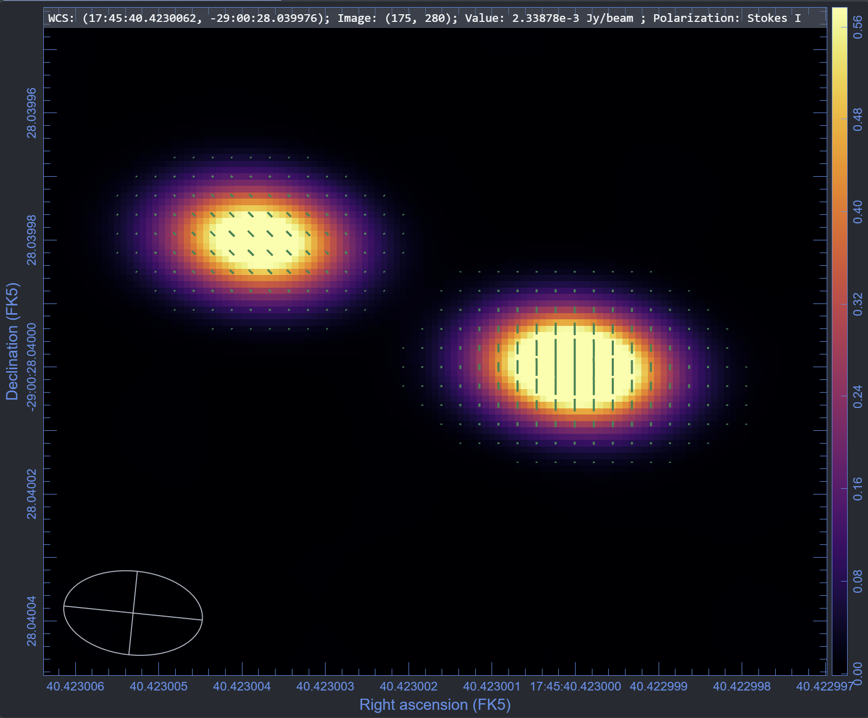
By setting $\texttt{CASE = 4}$ in the simulation script, we will generate the measurement set POLSIM_CASE_4.ms, corresponding to a double source (oriented with a position angle of about 45 degrees) with different Stokes parameters for each component. In this case, the instrumental polarization is assumed perfect.
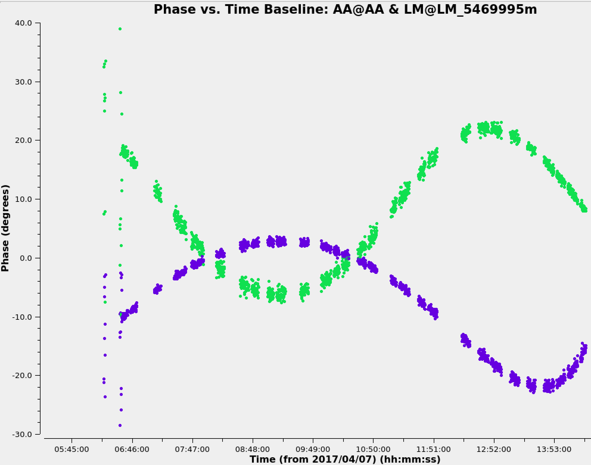
Run $\texttt{plotms}$ and generate plots of visibility amplitudes and phases for some prepresentative baselines, in both parallel-hand correlations (RR and LL) and cross-hand correlations (RL and LR). How do the RL visibilities compare to LR? Comment on the results in the frame of the Measurement Equation (and recalling the similar question about cross-hand phases made in $\texttt{CASE=2}$).
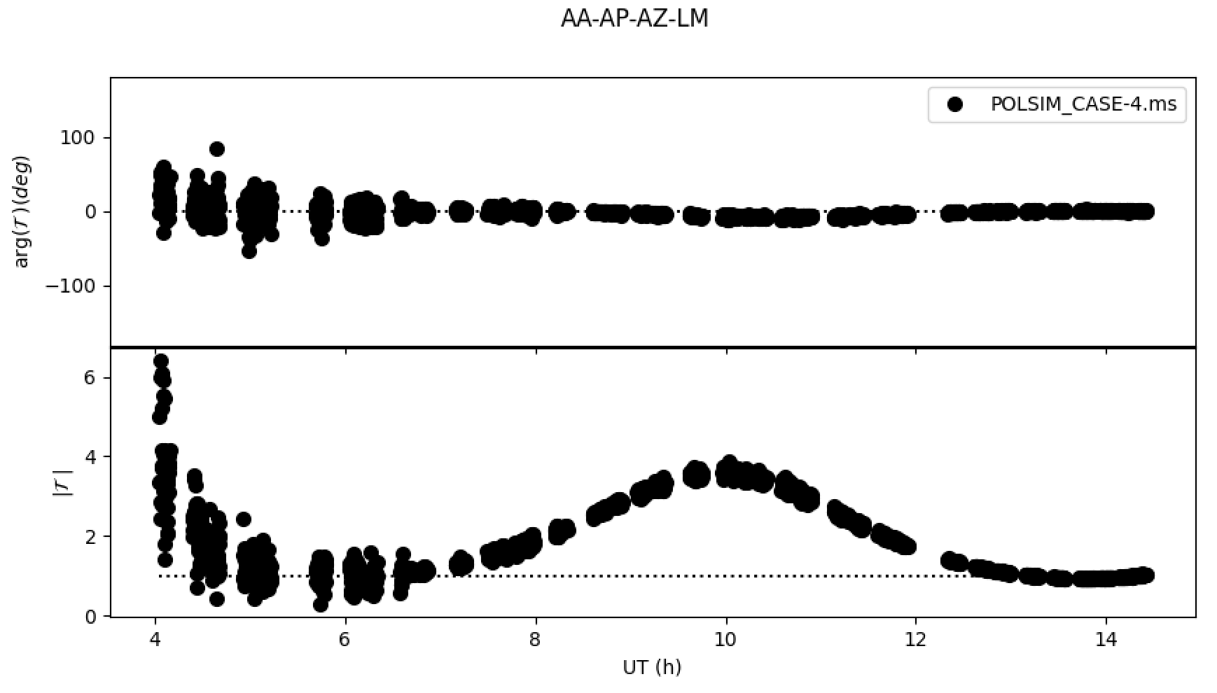
EXERCISE 2: Plot the closure traces for the quadruplet ALMA-APEX-LMT-SMT and compare them to those from the previous case. Comment on the results.
CASE=5. Polarized double source (with D-terms)
By setting $\texttt{CASE = 5}$ in the simulation script, we will generate the measurement set POLSIM_CASE_5.ms, corresponding to the same double source as in $\texttt{CASE = 4}$, but observed with an interferometer with imperfect instrumental polarization.
EXERCISE: Generate a full-polarization image from these data, but without any D-term calibration. Use $\texttt{iclean}$ and $\texttt{CARTA}$ and compare to the image obtained in the previous case. How do the polarization intensities and EVPA compare with the case of perfect instrumental polarization? How does the polarized image noise compare?
EXERCISE 2: Plot the closure traces for the quadruplet ALMA-APEX-LMT-SMT and compare with those from the previous case. Comment on the results.
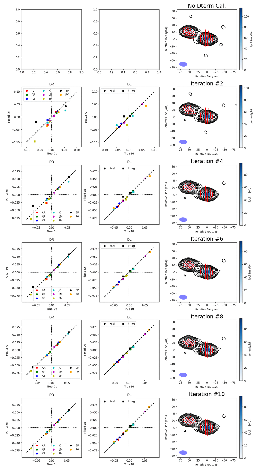
EXERCISE 3: Solve for the D-terms using the $\texttt{running_polsolve.py}$ script. How do the D-terms converge, compared to the case of a simple point-like structure?
CASE=6. Polarized point source (with cross-delay)
By setting $\texttt{CASE = 6}$ in the simulation script, we will generate the measurement set POLSIM_CASE_6.ms, corresponding to a polarized point source observed by an interferometer with instrumental polarization and non-zero cross-polarization delay. In this case, we will have to estimate the delay and apply it to the data, before attempting to calibrate the D-terms:
- Run $\texttt{gaincal}$ with $\texttt{gaintype='KCROSS'}$ (you may also set $\texttt{calmode='p'}$) and $\texttt{combine='scan'}$ (together with $\texttt{solint='inf'}$, since the R-L delay is constant). Setting ALMA as the reference antenna may also be a good option.
- Run $\texttt{applycal}$, to apply the cross-delay table and split the $\texttt{corrected}$ column into a new measurement set.
EXERCISE: Use the script $\texttt{running_polsolve.py}$ to solve for the D-terms, using the new measurement set (i.e., the one with the corrected cross-delay). Compare the final image (using, e.g., $\texttt{CARTA}$) to that of the previous case. Take a look at the correlation plots between fitted D-terms and their ground-truth values and comment on the results.
Part II: Real Data
EHT Observations of M87* in 2017
Let us run $\texttt{listobs}$ on the measurement set $\texttt{EHT-11Apr17_M87.ms}$, to check its contents:
================================================================================
           MeasurementSet Name:  /home/marti/WORK_LOCAL/ERIS_2026_POL/EHT_3601/EHT_11Apr2017_M87.ms      MS Version 2
================================================================================
   Observer: EHT     Project:
Observation: VLBA
Data records: 7447       Total elapsed time = 24938.6 seconds
   Observed from   11-Apr-2017/00:32:00.4   to   11-Apr-2017/07:27:39.0 (TAI)

   ObservationID = 0         ArrayID = 0
  Date        Timerange (TAI)          Scan  FldId FieldName             nRows     SpwIds   Average Interval(s)    ScanIntent
  11-Apr-2017/00:32:00.4 - 00:37:59.2     1      0 M87                         36  [0]  [9.21]
              00:41:00.2 - 00:46:59.8     2      0 M87                         42  [0]  [8.93]
              00:50:00.4 - 00:55:59.8     3      0 M87                        108  [0]  [9.1]
              01:15:00.8 - 01:20:59.9     4      0 M87                        108  [0]  [9.05]
              ...........
              06:40:00.2 - 06:45:59.8    20      0 M87                        540  [0]  [9.07]
              07:11:00.0 - 07:17:00.0    21      0 M87                        435  [0]  [9.06]
              07:25:00.2 - 07:27:39.0    22      0 M87                        160  [0]  [9.11]
           (nRows = Total number of rows per scan)
Fields: 1
  ID   Code Name                RA               Decl           Epoch   SrcId      nRows
  0         M87                 12:30:49.423382 +12.23.28.04366 J2000   0           7447
Spectral Windows:  (1 unique spectral windows and 1 unique polarization setups)
  SpwID  Name   #Chans   Frame   Ch0(MHz)  ChanWid(kHz)  TotBW(kHz) CtrFreq(MHz)  Corrs
  0      none       1   TOPO  227070.703   1856000.000   1856000.0 227070.7031   RR  RL  LR  LL
Sources: 1
  ID   Name                SpwId RestFreq(MHz)  SysVel(km/s)
  0    M87                 0     0              0
Antennas: 7:
  ID   Name  Station   Diam.    Long.         Lat.                Offset from array center (m)                ITRF Geocentric coordinates (m)
                                                                     East         North     Elevation               x               y               z
  0    AA    AA        25.0 m   -067.45.17.1  -22.53.27.9         -0.0000       -0.0000  6379959.6713  2225060.813600 -5440059.599940 -2481681.150540
  1    AP    AP        25.0 m   -067.45.32.9  -22.52.04.0         -0.0000       -0.0000  6379998.2522  2225039.529700 -5441197.629200 -2479303.359700
  2    AZ    AZ        25.0 m   -109.53.28.5  +32.31.37.1         -0.0000        0.0000  6375090.8598 -1828796.200000 -5054406.800000  3427865.200000
  3    JC    JC        25.0 m   -155.28.37.3  +19.42.01.7         -0.0000        0.0000  6379816.0683 -5464584.676000 -2493001.170000  2150653.982000
  4    LM    LM        25.0 m   -097.18.53.2  +18.52.04.0         -0.0000        0.0000  6380483.8311  -768715.632000 -5988507.072000  2063354.852000
  5    PV    PV        25.0 m   -003.23.33.4  +36.52.52.7         -0.0000        0.0000  6373329.0065  5088967.745440  -301681.185860  3825012.205610
6 SM SM 25.0 m -155.28.39.2 +19.42.06.6 -0.0000 0.0000 6379810.7485 -5464555.493000 -2492927.989000 2150797.176000These data have already been fringe-fitted, calibrated in amplitude, and self-calibrated in a careful process of hybrid imaging. Hence, instrumental polarization is the only remaining calibration step. For this, we will use the script $\texttt{EHT_ERIS26_polcal.py}$. The contents of this script are remarkably similar to those of $\texttt{running-polsolve.py}$, so we are not going to explain it again.
EXERCISE: Run $\texttt{polsolve}$ using the provided script, which will run the first imaging iteration using $\texttt{iclean}$. There, you will have to define the CLEAN masks, ensuring that you have the same exact masks for all the Stokes parameters. Once the iterations are finished, use $\texttt{CARTA}$ to generate a full-polarization image of M87*. You can also use the $\texttt{plotPolImage}$ function of $\texttt{casa-poltools}$, which will give you complementary information printed out in the terminal (i.e., peak polarization intensity, EVPA at the peak, and intensity-weighted EVPA).
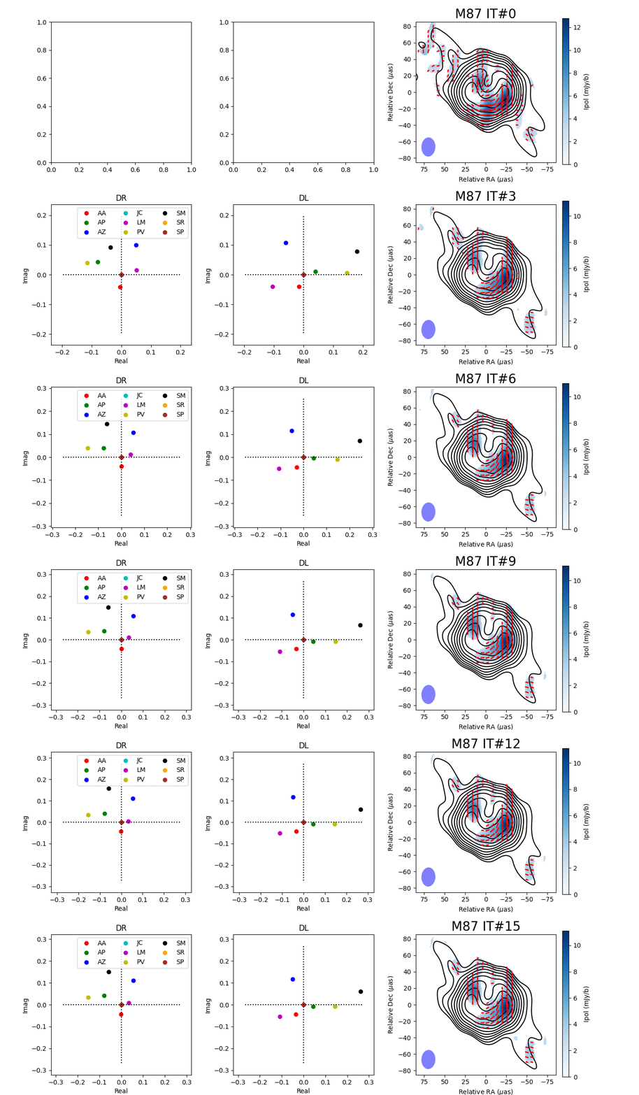
The residuals after proper D-term calibration are basically thermal noise, as you can check for the most sensitive EHT baselines in 2017 (i.e., those with ALMA) in these plots generated by $\texttt{polsolve}$ in the last iteration (left is data; right, residuals):

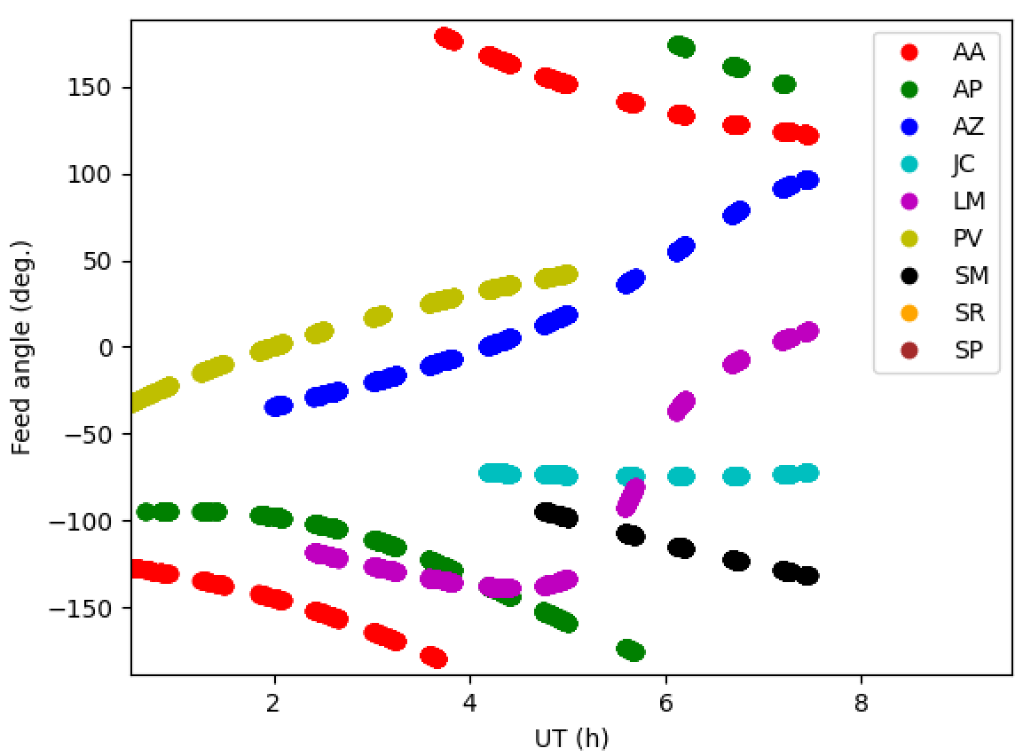
QUESTION: Take a look at the plot of feed angles vs. time generated by the script. The values for ALMA (AA) and APEX (AP) look quite different, despite the fact that they are very close geographically. How can you explain this?
VLBA Observations of 3C279 and OJ287 at 7mm
These data are part of project $\texttt{BG251A}$, which contains VLBA full-polarization observations of 3C279 and OJ287 at 7mm (43GHz). For this tutorial, we have already pre-calibrated the parallel-hand data in both phase and amplitude, so you don't have to worry about fringe-fitting and atmospheric opacity. We have splitted only four sources of the dataset (3C84, M84, OJ287 and 3C279). Run $\texttt{listobs}$ on the masurement set $\texttt{VLBA_BG251A_7mm.ms}$ and check the output:
 ================================================================================
           MeasurementSet Name:  /home/marti/WORK_LOCAL/ERIS_2026_POL/VLBA_7mm/VLBA_BG251A_7mm.ms      MS Version 2
================================================================================
   Observer: BG251A     Project:
Observation: VLBA
Data records: 317688       Total elapsed time = 35617 seconds
   Observed from   05-May-2017/23:16:29.0   to   06-May-2017/09:10:06.0 (UTC)

   ObservationID = 0         ArrayID = 0
  Date        Timerange (UTC)          Scan  FldId FieldName             nRows     SpwIds   Average Interval(s)    ScanIntent
  05-May-2017/23:16:29.0 - 23:17:25.0     1      0 3C84                      9696  [0,1,2,3,4,5,6,7]  [2, 2, 2, 2, 2, 2, 2, 2]
              23:18:43.0 - 23:23:35.0     2      0 3C84                     32376  [0,1,2,3,4,5,6,7]  [2, 2, 2, 2, 2, 2, 2, 2]
              23:30:05.0 - 23:32:01.0     3      1 OJ287                    16304  [0,1,2,3,4,5,6,7]  [2, 2, 2, 2, 2, 2, 2, 2]
  06-May-2017/00:09:56.0 - 00:11:52.0     4      1 OJ287                    16336  [0,1,2,3,4,5,6,7]  [2, 2, 2, 2, 2, 2, 2, 2]
  .......
              02:05:42.0 - 02:06:08.0    11      2 M84                       4256  [0,1,2,3,4,5,6,7]  [2, 2, 2, 2, 2, 2, 2, 2]
              02:39:35.0 - 02:41:31.0    12      1 OJ287                    20496  [0,1,2,3,4,5,6,7]  [2, 2, 2, 2, 2, 2, 2, 2]
              02:45:04.0 - 02:46:58.0    13      3 3C279                    20064  [0,1,2,3,4,5,6,7]  [2, 2, 2, 2, 2, 2, 2, 2]
  .......
              08:32:33.0 - 08:32:59.0    35      2 M84                       2064  [0,1,2,3,4,5,6,7]  [2, 2, 2, 2, 2, 2, 2, 2]
              09:08:12.0 - 09:10:06.0    36      3 3C279                    12456  [0,1,2,3,4,5,6,7]  [2, 2, 2, 2, 2, 2, 2, 2]
           (nRows = Total number of rows per scan)
Fields: 4
  ID   Code Name                RA               Decl           Epoch   SrcId      nRows
  0         3C84                03:19:48.160094 +41.30.42.10414 J2000   0          42072
  1         OJ287               08:54:48.874926 +20.06.30.64088 J2000   1         106200
  2         M84                 12:25:03.743335 +12.53.13.13928 J2000   2          66160
  3         3C279               12:56:11.166568 -05.47.21.52500 J2000   3         103256
Spectral Windows:  (8 unique spectral windows and 1 unique polarization setups)
  SpwID  Name   #Chans   Frame   Ch0(MHz)  ChanWid(kHz)  TotBW(kHz) CtrFreq(MHz)  Corrs
  0      none      16   TOPO   43024.875      2000.000     32000.0  43039.8750   RR  RL  LR  LL
  1      none      16   TOPO   43056.875      2000.000     32000.0  43071.8750   RR  RL  LR  LL
  2      none      16   TOPO   43088.875      2000.000     32000.0  43103.8750   RR  RL  LR  LL
  3      none      16   TOPO   43120.875      2000.000     32000.0  43135.8750   RR  RL  LR  LL
  4      none      16   TOPO   43152.875      2000.000     32000.0  43167.8750   RR  RL  LR  LL
  5      none      16   TOPO   43184.875      2000.000     32000.0  43199.8750   RR  RL  LR  LL
  6      none      16   TOPO   43216.875      2000.000     32000.0  43231.8750   RR  RL  LR  LL
  7      none      16   TOPO   43248.875      2000.000     32000.0  43263.8750   RR  RL  LR  LL
Sources: 32
  ID   Name                SpwId RestFreq(MHz)  SysVel(km/s)
  0    3C84                0     0              0
.......
  1    OJ287               0     0              0
.......
  2    M84                 0     0              0
.......
  3    3C279               0     0              0
.......
Antennas: 10:
  ID   Name  Station   Diam.    Long.         Lat.                Offset from array center (m)                ITRF Geocentric coordinates (m)
                                                                     East         North     Elevation               x               y               z
  0    BR    BR        25.0 m   -119.40.59.8  +47.56.23.6         -0.0000        0.0000  6366573.1559 -2112065.270560 -3705356.502585  4726813.644675
  1    FD    FD        25.0 m   -103.56.41.4  +30.27.59.8         -0.0000        0.0000  6374225.1305 -1324009.382231 -5332181.952615  3231962.375184
  2    HN    HN        25.0 m   -071.59.11.7  +42.44.30.3         -0.0000        0.0000  6368555.4400  1446374.797314 -4447939.684001  4322306.202257
  3    KP    KP        25.0 m   -111.36.44.7  +31.47.01.6         -0.0000        0.0000  6374084.6483 -1995678.899870 -5037317.693369  3357327.998305
  4    LA    LA        25.0 m   -106.14.44.2  +35.35.34.2         -0.0000        0.0000  6372831.2532 -1449752.646436 -4975298.573311  3709123.825446
  5    MK    MK        25.0 m   -155.27.19.9  +19.40.44.8         -0.0000        0.0000  6379464.1022 -5464075.247410 -2495247.833469  2148297.505345
  6    NL    NL        25.0 m   -091.34.26.9  +41.34.49.1         -0.0000        0.0000  6368913.6411  -130872.566143 -4762317.086160  4226850.992106
  7    OV    OV        25.0 m   -118.16.37.4  +37.02.47.3         -0.0000        0.0000  6371546.5879 -2409150.482445 -4478573.089077  3838617.324039
  8    PT    PT        25.0 m   -108.07.09.1  +34.07.19.7         -0.0000        0.0000  6373749.2196 -1640954.001748 -5014816.024612  3575411.768974
  9    SC    SC        25.0 m   -064.35.01.1  +17.38.42.4         -0.0000        0.0000  6376148.0958  2607848.668864 -5488069.494717  1932739.786060
Given that the measurement set contains several sources, the script $\texttt{VLBA_ERIS2026_polsolve.py}$ has the possibility of selecting different (sets of) calibrator(s) and target(s). We are going to use different combinations of calibrators, in order to check how this affects the estimated D-terms.
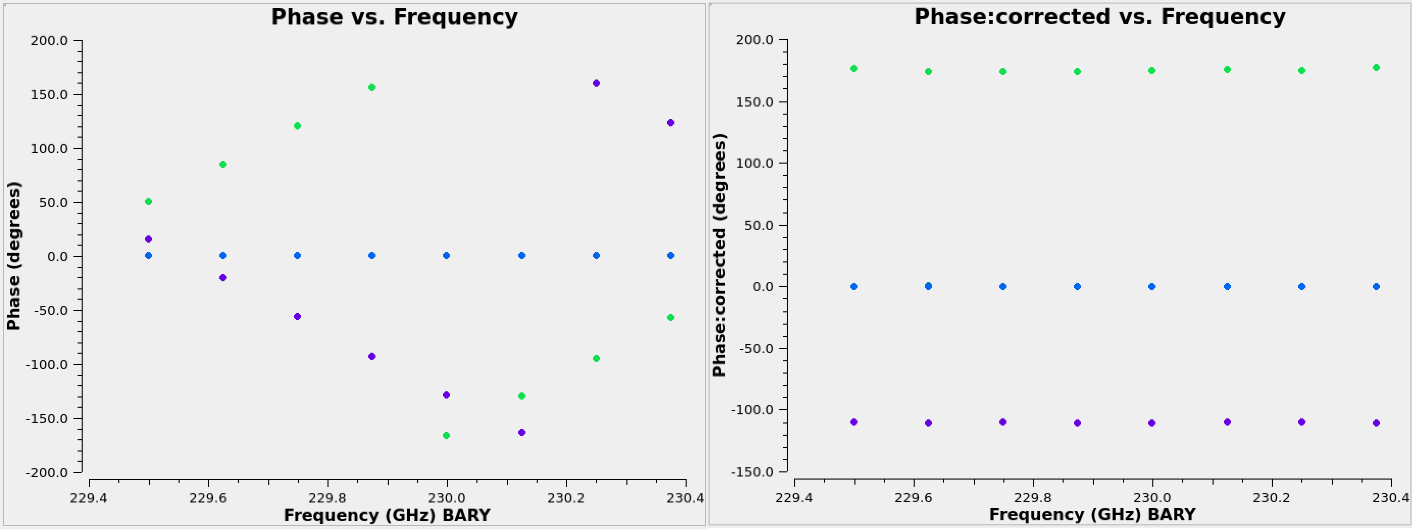
But before starting to calibrate the D-terms, we must calibrate the cross-polarization delay (and phase) of the reference antenna that we have used in the Global Fringe Fitting (Los Alamos, LA). The fringe fitting only cares about the parallel-hand correlations, RR and LL, which means that the relative instrumental delay (and phase) between the R and L polarization channels of Los Alamos (LA) are still affecting all the cross-hand data (i.e., all baselines are affected by the same cross-hand delay and phase). This delay can be easily seen by just plotting the cross-hand phases of any baseline with a good SNR (say, LA-KP or LA-FD, observing 3C279). Please, run $\texttt{plotms}$ and check it:

How do we estimate these instrumental cross-polarization delays? It has to be done in different steps. First, we will estimate the cross-hand single-band delays (SBD). Then, we will adjust the remaining phase slope across spectral windows (multi-band delays). Let's go step by step:
- Use $\texttt{gaincal}$ to determine the cross-hand SBDs:
gaincal(vis='VLBA_BG251A_7mm.ms',
        caltable='BG251A.KcrossSBD',
        gaintype='KCROSS', combine='scan',
        field='3C279', refant='LA')
Notice that we are not providing any polarization source model to $\texttt{gaincal}$ (it has no effect when we run it in $\texttt{KCROSS}$ mode). - Apply the table (using $\texttt{applycal}$; you will have to sort out how to do it, ensuring that $\texttt{parang}$ is always False) and check the $\texttt{corrected}$ data column in $\texttt{plotms}$. It should look like this:

As you can see, there is still a small slope of the cross-hand phases as a function of frequency (i.e., a small MBD). The easiest way to handle it would be to run $\texttt{polcal}$ with $\texttt{poltype='X'}$ (by undoing the parallactic-angle correction first, as we discussed in the first part of the tutorial). However, the $\texttt{polcal}$ algorithm fails to solve this particular problem. We will thus take a different strategy within $\texttt{CASA}$. - Combine the different spectral windows into one, so we can use $\texttt{gaincal}$ in $\texttt{KCROSS}$ mode again, this time to derive the cross-hand MBD.
mstransform(vis='VLBA_BG251A_7mm.ms',
            outputvis='VLBA_BG251A_7mm_spwComb.ms'
            datacolumn='corrected', combinespws=True,
            chanaverage=True, chanbin = 16,
            timeaverage=True,timebin='20s')
Notice that, besides combining the spectral windows, we are also averaging them in frequency (down to one channel per spectral window). This way, we avoid re-introducing small SBDs when applying the MBD correction to the whole band. We also average a bit in time, to help accelerate the CLEAN major cycles when we do the imaging. - Compute the cross-polarization MBD:
gaincal(vis='VLBA_BG251A_7mm_spwComb.ms',
        caltable='BG251A.KcrossMBD',
        gaintype='KCROSS', combine='scan',
        field='3C279', refant='LA')
- Apply the table to $\texttt{VLBA_BG251A_7mm_spwComb.ms}$ and check the $\texttt{corrected}$ data column. Now, the cross-hand phases look much flatter (not perfect, though). Notice that the absolute EVPA is not calibrated at this point, since we haven't had the chance to set a polarization model for the calibrator, 3C279. We will have to deal with the EVPA calibration later.

- Since $\texttt{polsolve}$ cannot pre-calibrate the data using $\texttt{CASA}$ tables on-the-fly, we need to $\texttt{split}$ the $\texttt{corrected}$ column of $\texttt{VLBA_BG251A_7mm_spwComb.ms}$, to generate a new measurement set that includes all these calibration steps. Let's call this new measurement set $\texttt{BG251A_kcrossCalib.ms}$:
split(vis='VLBA_BG251A_7mm_spwComb.ms',
      outputvis='BG251A_kcrossCalib.ms',
      datacolumn='corrected')
The $\texttt{VLBA_ERIS2026_polsolve.py}$ script will estimate the D-terms in the same way as we did in the previous cases (i.e., by an iterative self-calibration process, where a CLEAN model obtained from D-term calibrated data is used as the input for the next D-term estimates).
Using 3C279 as Polarization Calibrator
Open the script $\texttt{VLBA_ERIS2026_polsolve.py}$ and edit its header to set $\texttt{3C279}$ as the $\texttt{field}$ (i.e., $\texttt{field='3C279'}$). You can add more sources to $\texttt{target_field}$ (separated by commas) if you want to image them using the D-terms estimated from 3C279. For instance, $\texttt{target_field='M84'}$ will calibrate M84 using the D-terms derived from 3C279.
The first time that you run the script with a given calibrator source, $\texttt{iclean}$ will be run at the beginning, so you can set its CLEAN masks. Then, after that, all the further deconvolutions of that source will use the same mask and everything will run automatically.
NOTE: you can also play with the CLEAN parameters (like the weighting, which you could set to $\texttt{natural}$ instead of $\texttt{uniform}$).

After the last iteration, write down the EVPA values of 3C279 printed by $\texttt{plotPolImage}$ on the terminal (i.e., the values for $\texttt{EVPA(Peak)}$ and $\texttt{EVPA(avg)}$). You will need these values later, for the absolute EVPA calibration.
Take a look at the plots of visibility residuals in phasor space (for all the baselines related to Los Alamos, these will be in the file $\texttt{BG251A_kcrossCalib_PolSolve_Residuals_AA.png}$) and the actual visibilities in the same space (file $\texttt{BG251A_kcrossCalib_PolSolve_Data_AA.png}$ for Los Alamos) and comment on the results.

Using OJ287 as Polarization Calibrator
Open the script $\texttt{VLBA_ERIS2026_polsolve.py}$ in an editor and set $\texttt{field='OJ287'}$. Then, run the script. After setting the masks with $\texttt{iclean}$, the script will take a bit of time to recover D-term estimates that should be close to these ones:

We can compare the D-terms estimated using 3C279 as calibrator to those using OJ287. In principle, if the calibration is OK, both sets of D-terms should be similar. Let us check this by running the function $\texttt{compareDterms}$ (from the $\texttt{poltools_helper}$ module), in a way similar to what we did with the simulated data (CASE=3).
from poltools_helper import compareDterms
compareDterms(dt1='3C279.polsolve-dterms',dt2='OJ287.polsolve-dterms')
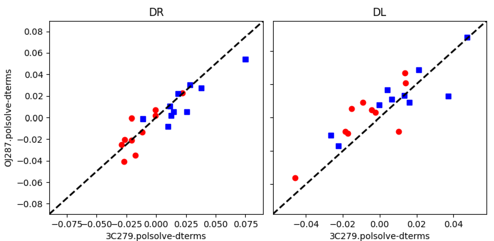
There is definitely a correlation between the D-terms estimated using 3C279 and those estimated using OJ287. This is a good indicative that we are doing things properly!
Using 3C84 as Polarization Calibrator
Even tough the D-terms using 3C279 and OJ287 look similar, the case of 3C84 is quite different. Run the calibration script using 3C84 as the $\texttt{field}$ and $\texttt{target_field}$. Then, generate the correlation plot between the D-terms using 3C84 and 3C279. It should be similar to this one:
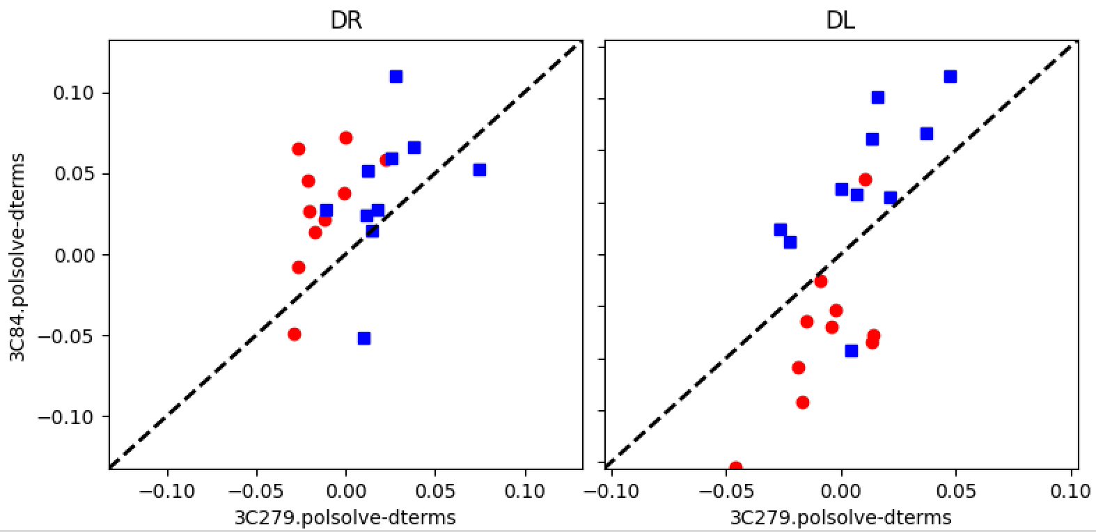
QUESTION: What could be the reason for such a big discrepancy between the D-terms using 3C84 and those using 3C279 and/or OJ287? A look at the plot of elevation (or feed angle) vs. time for all these sources may help you answer the question.
EXERCISE: 3C84 is quite compact (even with VLBI at 7mm) and basically unpolarized. Hence, we could run $\texttt{polsolve}$ by forcing the source model to be that of an unpolarized point source. With this assumption, just one scan of 3C84 should suffice to derive pretty decent D-terms. Let's do this with this line of code (the peak intensity of 3C84 is about 3.8 Jy; you can check it in different ways with CASA):
polsolve(vis='POLSIM_CASE-3.ms', caltable='3C84_unpol.polsolve',
         CLEAN_models=[3.8], frac_pol=[0.0], EVPA=[0.0], PolSolve=[False])
This code asks $\texttt{polsolve}$ to fit only for the D-terms and force the source model to be fixed (i.e., $\texttt{PolSolve=[False]}$) and unpolarized (i.e., $\texttt{frac_pol=[0.0]}$). After running it, please generate the correlation plot between the new D-terms and those derived from 3C279 and/or OJ287. The plot should look like this one:
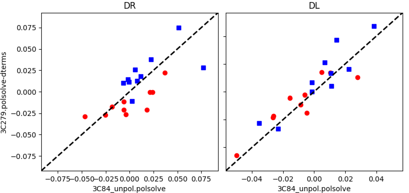
Now, it doesn't look that bad!
Using M84 as Polarization Calibrator
If you plot some visibilities of M84, you will see that the SNR is quite low, compared to what a calibrator source should look like. Thus, we will not show the results for M84 in this tutorial, although you are encouraged to play with it, if you like. In any case, don't expect good results.
Using 3C279 and OJ287 simultaneously
By setting $\texttt{field='3C279,OJ287'}$ in the calibration script, we will use both calibrator sources simultaneously, in a self-consistent D-term fitting. Run the script in this mode and compare the D-terms to those estimated above.

EXERCISE: Plot the correlation between the D-terms calibrated in this section and the D-terms estimated using each calibrator independently. Is there any calibrator dominating the solution? Which one?
OPTIONAL EXTRA EXERCISE: Repeat the calibration by adding also 3C84 (and/or M84 as well). Does the addition of these sources affect the quality of the fit? Comment on the results.
Absolute EVPA calibration
The only remaining quantity to be calibrated in our data is the absolute EVPA, which appears as a constant phase offset between the R and L polarization channels of all antennas (i.e., the same quantity has to be added to all baselines, in the exact same way). Therefore, all the polarization images generated in the previous steps have been more or less correct, regarding the polarization intensities and the relative polarization angles. However, all these EVPAs still have to be corrected by a global constant.
If at least one of the observing antennas had a linear-polarization feed, the absolute EVPA would be automatically calibrated by just using that antenna as the reference in the process of fringe fitting (we wouldn't even need to calibrate the "$\texttt{KCROSS}$" cross-hand delay and phase!). This is the case of the Event Horizon Telescope (which uses ALMA as the reference antenna) and the M87 data analyzed a few sections above. However, all the VLBA antennas have circular feeds, so we need to estimate the absolute EVPA by comparison of the average polarization angle of a calibrator with some other independent measurement of the same source, close in both time and frequency. The source 3C279 is well monitored by the Blazars Research Group of Boston University. Indeed, their monitoring of 3C279 at the wavelength of 7mm is pretty good. Their closest EVPA measurement to our epoch of observations gives a value of 52 degrees.
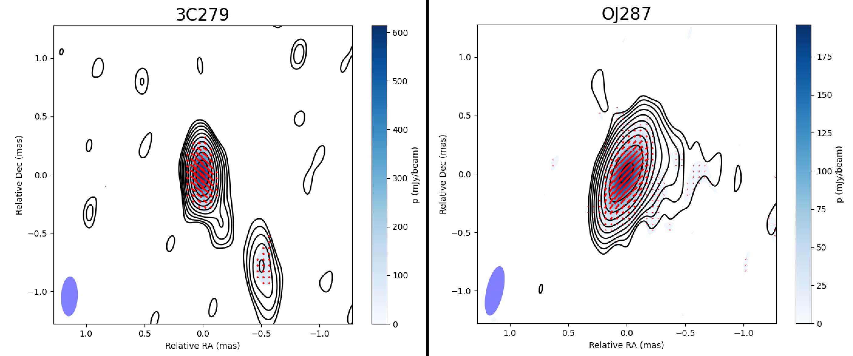
EXERCISE: Get the average EVPA of 3C279 estimated by $\texttt{plotPolImage}$ from our data (i.e., the value $\texttt{EVPA(avg)}$ that was printed on the terminal and you wrote down a few minutes ago) and compute the difference between that value and the true EVPA of 3C279 (52 degrees). Then, use this difference to generate corrected EVPA images for 3C279 and OJ287. You can do this in different ways:
- Using $\texttt{CARTA}$. There is an option in the GUI that allows you to rotate all the EVPAs in a plot.
- Using $\texttt{plotPolImage}$ (from the $\texttt{poltools_helper}$ module). The keyword $\texttt{rotateEVPA}$ is what you need here. In this case, for 3C279, we will run these lines ($\texttt{EROT}$ is the EVPA rotation that we need to apply, in degrees):
from poltools_helper import plotPolImage plotPolImage(img='3C279.image', mSigmaCut=1.25, SigmaCut=2.0, dPol=20, lPol=0.05, rotateEVPA = EROT) - Correcting the R-L phases of all baselines (either manually or via a $\texttt{CASA}$ table), to reflect this rotation in the data (this is the somewhat hardest way). If you prefer this option, these lines of code may help you ($\texttt{EROT_RAD}$ is the rotation angle, in radians):
tb.open("BG251A_kcrossCalib.ms",nomodify=True)
DATA = tb.getcol("DATA")
DATA[1,:,:] *= np.exp(2.*1.j*EROT_RAD)  # This is RL
DATA[2,:,:] *= np.exp(-2.*1.j*EROT_RAD) # This is LR
tb.putcol("DATA",DATA)
tb.close()
After running these lines, the visibilities will be corrected for the absolute EVPA. Then, re-running the calibration and imaging scripts will give you the final images.
Additional Material
Additional Activities
Suggestions for further work:
A. These data:
- Estimate the errors in the polarisation images of 3C279 and OJ287, from the images and/or analytically.
- Experiment with the different weightings and imaging parameters as at the end of the imaging and self-calibration tutorials, but in full polarisation.
B. Look at the polarisation CASA guides: