VLBI Self-calibration & Imaging
For this section, we will work with two dataset from the European VLBI Network (EVN). The first dataset is from the blazar Mrk 501, observed at X-band (8 GHz) with the EVN in October 2025 (project code EE010). The second dataset is a phase-referencing project (project code RSM07) observed on 16 September 2025 at L-band (1.67 GHz). The general calibration and imaging steps required for VLBI data are similar to what was covered in the previous tutorial about calibration, imaging and self-calibration. However, there are some important differences that will be pointed out in this tutorial.
A few words about VLBI Calibration
For the sake of time, we will not cover VLBI calibration in detail. If you are interested in the details of VLBI calibration, please have a look at this EVN tutorial, where all required calibration steps are explained. One important difference to the previous calibration tutorial presented at this ERIS is that fringe-fitting is an integral part of VLBI phase calibration, as independent clocks from antennas that are thousands of kilometers apart from each other have to be aligned. If you are interested in trying out the calibration yourself, you can download the raw data for RSM07 from the EVN archive (under "Fitsfiles") and execute the calibration script that we have prepared for you in CASA (you will also need this flag file in your working directory).
execfile('calibrate.py')
Data required
For this tutorial, we have already prepared and calibrated two datasets for you. You will require the following files, which are bundled together in the archive linked below.
MRK501_calibrated.ms- measurement set containing the calibrated visibilities of Mrk 501 (from EE010)J1848+3219_calibrated.ms- measurement set containing the calibrated visibilities of the RSM07 phase reference calibrator (J1848+3219).3C395_calibrated.ms- measurement set containing the calibrated visibilities of the RSM07 phase reference target (3C395).
We also provide an archive with the full solution (incl. images and self-calibration tables), in case you get stuck somewhere.
Table of contents
Part 1: Imaging and self-calibration of Mrk 501 (EE010)
- Inspect the data
- Imaging the source
- Phase-Self Calibration
- Imaging the source again
- Amplitude Self-Calibration and Final Imaging
Part 2: Imaging and self-calibration of a phase referencing observation (RSM07)
Part 1: Imaging and self-calibration of Mrk 501 (EE010)
1. Inspect the data
In order to familiarize yourself with the data it is a good idea to execute some of the standard procedures shown in the introduction tutorial. We will not replicate all steps here, but let's at least have a look at the uv-coverages of both sources and the amplitudes and phases vs. uv-distance.
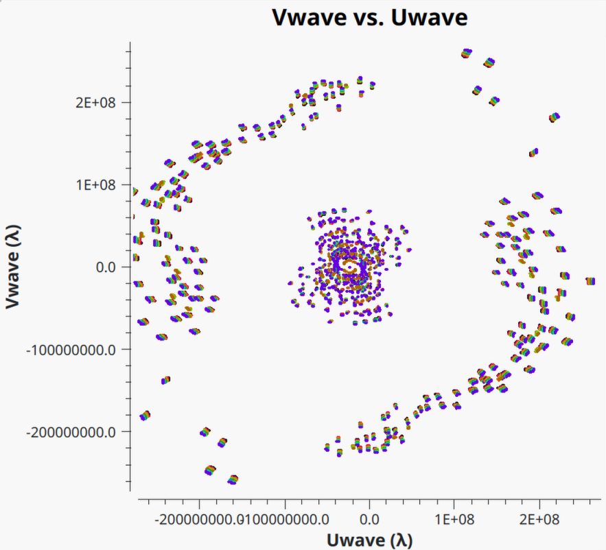
- First let's have a look at the uv-coverage, using
plotms()plotms( vis="MRK501_calibrated.ms/", xaxis="uwave", yaxis="vwave", coloraxis="spw" ) - Then let us check the visibility amplitudes and phases vs. uv-distance
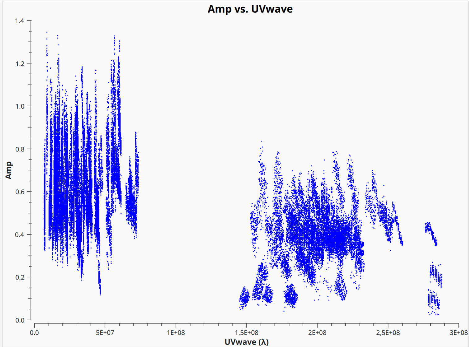
plotms(
	vis="3C395_calibrated.ms/",
	xaxis="uvdist",
	yaxis="amp",
	correlation="rr,ll"
	)
plotms(
	vis="3C395_calibrated.ms/",
	xaxis="uvdist",
	yaxis="phase",
	correlation="rr,ll"
	)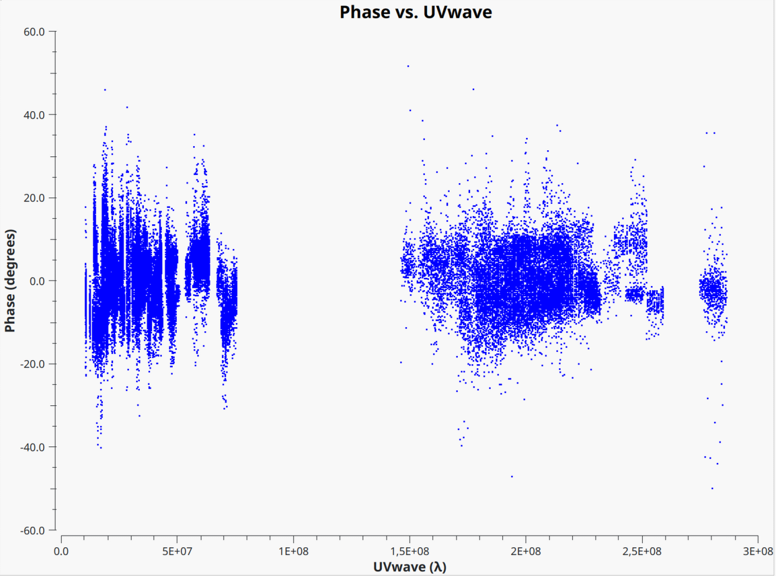
You can clearly see that the scatter in phase and amplitudes is still quite high, which we will try to improve through self-calibration in the following steps.
Note: For typical VLBI data, you will likely have to go through some additional flagging. We have already taken care of flagging the data provided here, so you can skip the flagging process.
2. Imaging the source
Before we can perform any kind of self-calibration, we first need to obtain an initial image. Since the observed source is bright enough, we can directly start with imaging it and later use it to derive the self-calibration solutions.
- Let's recall the
tcleantask from the previous tutorials (oricleanfor MacOS), to create a first image.Linuxtclean( vis="MRK501_calibrated.ms/", imagename="MRK501_first_image", specmode="mfs", niter=1500, cycleniter=300, threshold=0, imsize=[1024,1024], cell="0.1mas", weighting="natural", deconvolver="hogbom", savemodel="modelcolumn", interactive=True )MacOSiclean( vis="MRK501_calibrated.ms/", imagename="MRK501_first_image", specmode="mfs", niter=1500, cycleniter=300, threshold=0, imsize=[1024,1024], cell="0.1mas", weighting="natural", deconvolver="hogbom", savemodel="modelcolumn" ) ft(vis="MRK501_calibrated.ms/", model="MRK501_first_image.model", usescratch=True ) Let's start with a first clean mask similar to this
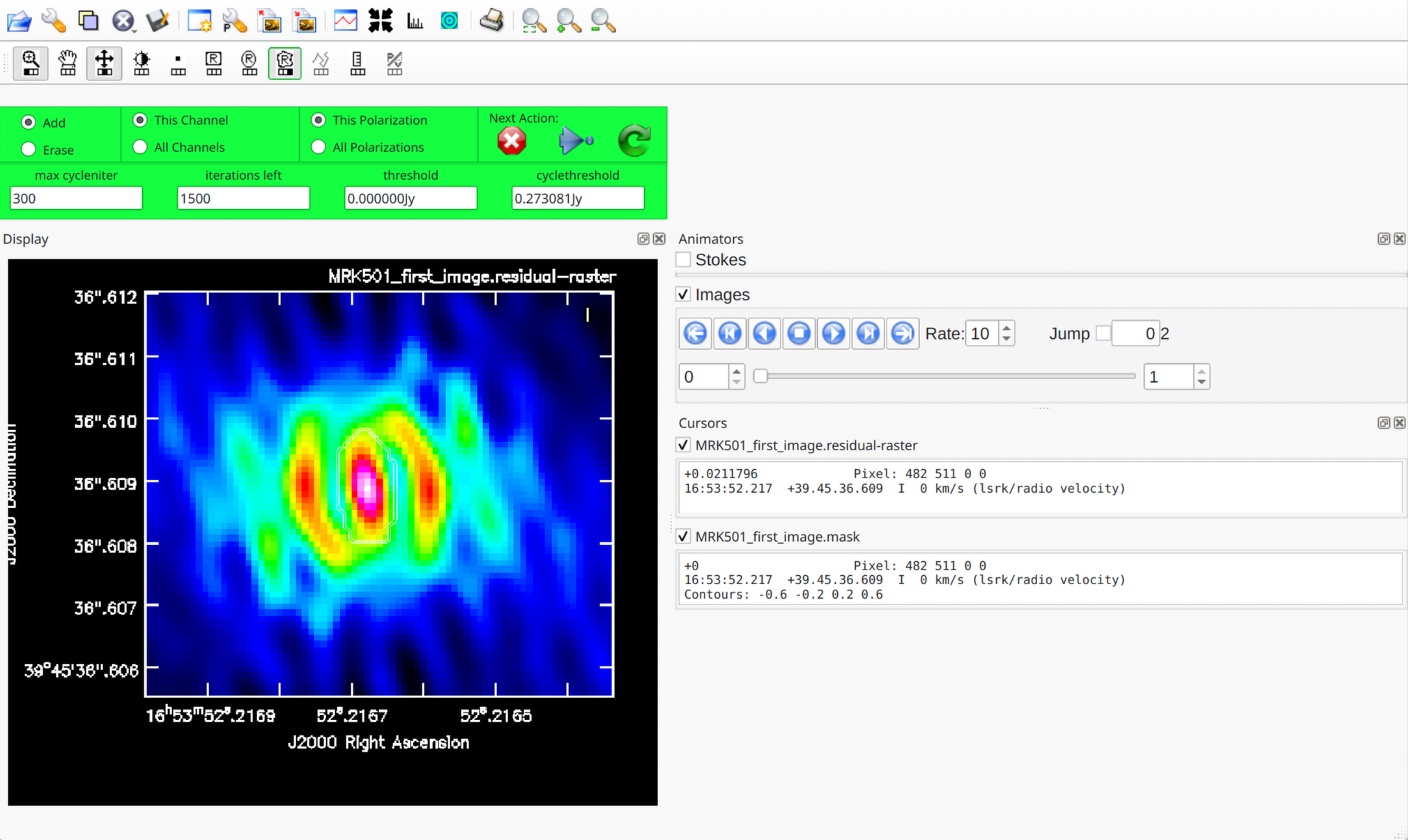
Keep cleaning and adjusting the mask (if required) until your residual map looks similar to this:
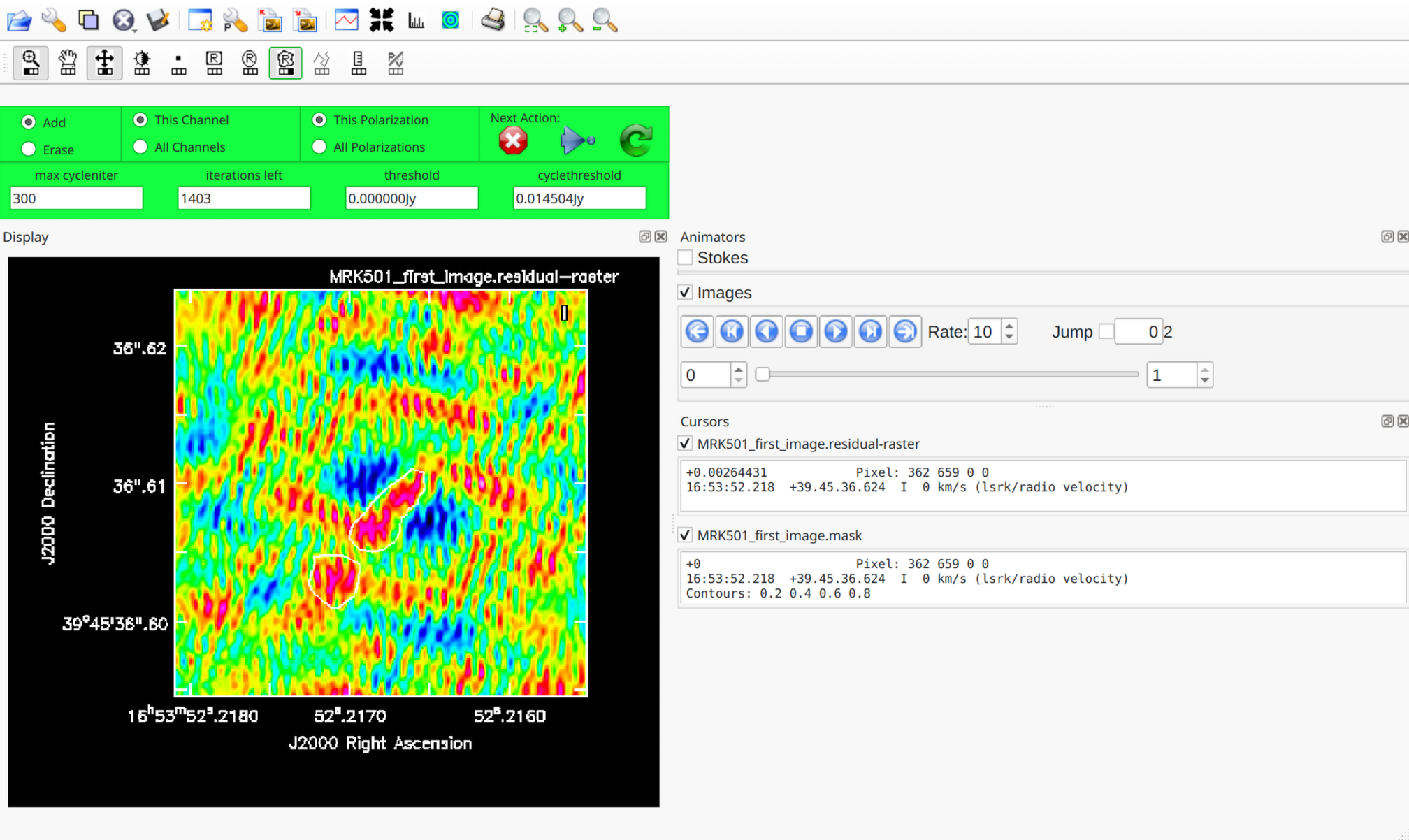
- Now you can close the
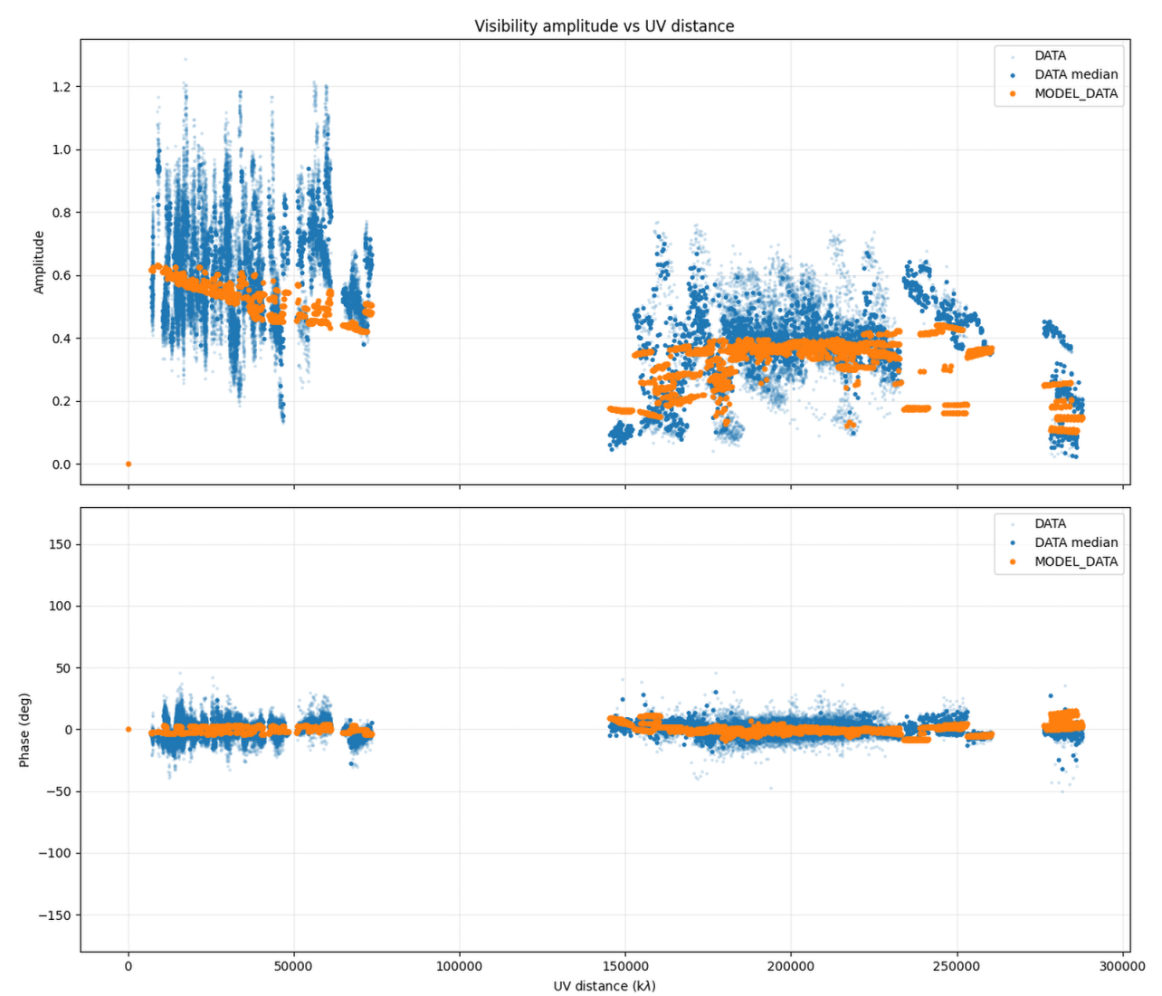
tcleanwindow by clicking on the large X. It may take some time as CASA is loading your model into the measurement set. Once this process has finished it is a good idea to check that the CLEAN model that was created describes the data reasonably well. Unfortunately, there is no built-in CASA plot function to do this, but we have created a short plotting script that you may run on your measurement set to compare its model and data visibilities.execfile("compare_model_data.py")The output should look something like this and the CLEAN model should describe the data reasonably well.
3. Phase Self-Calibration
Once you are satisfied with your initial CLEAN image and the model visibilities describe the data as good as possible, we can start with deriving self-calibration solutions.
-
First, we will start with a phase self-calibration and use a long solution interval
gaincal( vis="MRK501_calibrated.ms/", calmode="p", #use "p" to calibrate phases only or "ap" for amplitude and phase caltable="MRK501-sc-p1", field="1653+3945", solint="10min", refant="EF", minblperant=3, minsnr=5 ) -
Now that we created a first phase self-calibration table, we can plot it
and look at the suggested corrections
plotms(
	vis="MRK501-sc-p1",
	gridcols=2,
	gridrows=3,
	xaxis="time",
	yaxis="phase",
	iteraxis="antenna",
	coloraxis="spw",
	plotrange=[-1,-1,-180,180]
	)
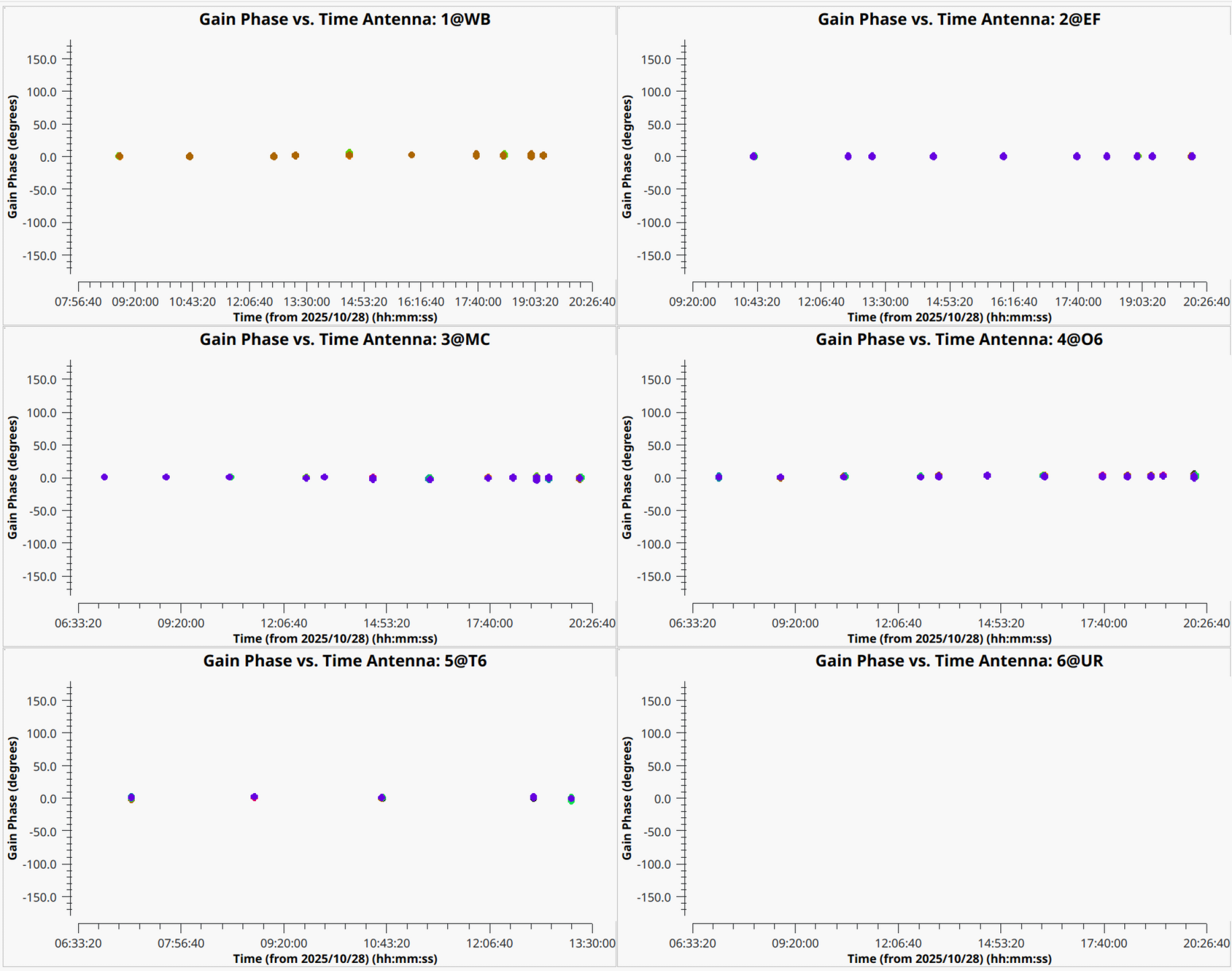
The plot should look similar to the one shown below. Note that the corrections are typically small. Additionally, for some antennas the solution is missing because they have no data or were already flagged. This is fine and you do not have to worry about it.
-
Finally, the self-calibration needs to be applied to the measurement set, using the
applycaltaskapplycal( vis="MRK501_calibrated.ms/", gaintable=["MRK501-sc-p1"], )
4. Iterative self-cal and imaging (hybrid imaging)
After applying the first phase self-calibration, you should go back to step 2
and create a new image of the phase calibrator (ideally, use a different imagename
value for tclean, otherwise you will run into an error).
Once this is done, you can perform self calibration in phase again, but with a shortened solution interval
(2min, as you do not expect faster changes due to the atmosphere).
After another imaging round, if the solutions (in plots) seem to converge to just small improvements,
one can run the self-calibration in amplitude and phase (using calmode="ap" in
gaincal).
For amplitude self-calibration, the fastest changes you expect are probably on the order of a few minutes for this dataset.
Therefore, a solution interval of a few minutes is sufficient. You can consider calibrating with a longer solution interval first,
and then lower the solution interval gradually. Below, we provide a short summary of these steps
-
Image Mrk 501 again
Linuxtclean( vis="MRK501_calibrated.ms/", imagename="MRK501_second_image", specmode="mfs", niter=1500, cycleniter=300, threshold=0, imsize=[1024,1024], cell="0.1mas", weighting="natural", deconvolver="hogbom", savemodel="modelcolumn", interactive=True )MacOSiclean( vis="MRK501_calibrated.ms/", imagename="MRK501_second_image", specmode="mfs", niter=1500, cycleniter=300, threshold=0, imsize=[1024,1024], cell="0.1mas", weighting="natural", deconvolver="hogbom", savemodel="modelcolumn" ) ft(vis="MRK501_calibrated.ms/", model="MRK501_second_image.model", usescratch=True ) -
Compare model with data
execfile("compare_model_data.py") -
Generate phase calibration table with shorter solution interval of 2 minutes.
gaincal( vis="MRK501_calibrated.ms/", calmode="p", #use "p" to calibrate phases only or "ap" for amplitude and phase caltable="MRK501-sc-p2", field="J1653+3945", solint="2min", gaintable="MRK501-sc-p1", interp=["linear"], refant="EF", minblperant=3, minsnr=5 ) -
Apply both phase calibration tables to the data
applycal( vis="MRK501_calibrated.ms/", gaintable=["MRK501-sc-p1","MRK501-sc-p2"] ) -
Image Mrk 501 again
Linuxtclean( vis="MRK_calibrated.ms/", imagename="MRK501_third_image", specmode="mfs", niter=1500, cycleniter=300, threshold=0, imsize=[1024,1024], cell="0.1mas", weighting="natural", deconvolver="hogbom", savemodel="modelcolumn", interactive=True )MacOSiclean( vis="MRK501_calibrated.ms/", imagename="MRK501_third_image", specmode="mfs", niter=1500, cycleniter=300, threshold=0, imsize=[1024,1024], cell="0.1mas", weighting="natural", deconvolver="hogbom", savemodel="modelcolumn" ) ft(vis="MRK501_calibrated.ms/", model="MRK501_third_image.model", usescratch=True ) -
Compare model with data
execfile("compare_model_data.py") -
Generate calibration table for amplitude and phase self-calibration.
gaincal( vis="MRK501_calibrated.ms/", calmode="ap", #use "p" to calibrate phases only or "ap" for amplitude and phase caltable="MRK501-sc-ap", field="1653+3945", solint="30min", gaintable=["MRK501-sc-p1","MRK501-sc-p2"], interp=["linear","linear"], refant="EF", minblperant=3, minsnr=5 ) -
Apply all self-calibration tables to the data
applycal( vis="MRK501_calibrated.ms/", gaintable=["MRK501-sc-p1","MRK501-sc-p2","MRK501-sc-ap"], ) -
Finally, you can image the phase calibrator one last time, to obtain a final image
Linux
tclean( vis="MRK501_calibrated.ms/", imagename="MRK501_final_image", specmode="mfs", niter=1500, cycleniter=300, threshold=0, imsize=[1024,1024], cell="0.1mas", weighting="natural", deconvolver="hogbom", savemodel="modelcolumn", interactive=True )MacOSiclean( vis="MRK501_calibrated.ms/", imagename="MRK501_final_image", specmode="mfs", niter=1500, cycleniter=300, threshold=0, imsize=[1024,1024], cell="0.1mas", weighting="natural", deconvolver="hogbom", savemodel="modelcolumn" ) ft(vis="MRK501_calibrated.ms/", model="MRK501_final_image.model", usescratch=True ) -
You can inspect your final image with
imviewand it will likely look similar to this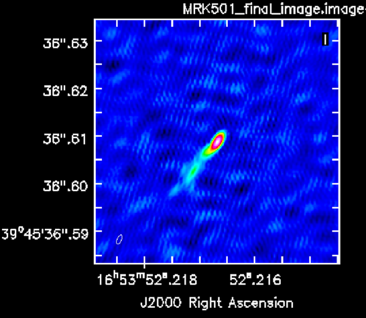
Part 2: Imaging and self-calibration of a phase referencing observation
1. Inspect the data
In order to familiarize yourself with the data it is a good idea to execute some of the standard procedures shown in the introduction tutorial. We will not replicate all steps here, but let's at least have a look at the uv-coverages of both sources and the amplitudes and phases vs. uv-distance.
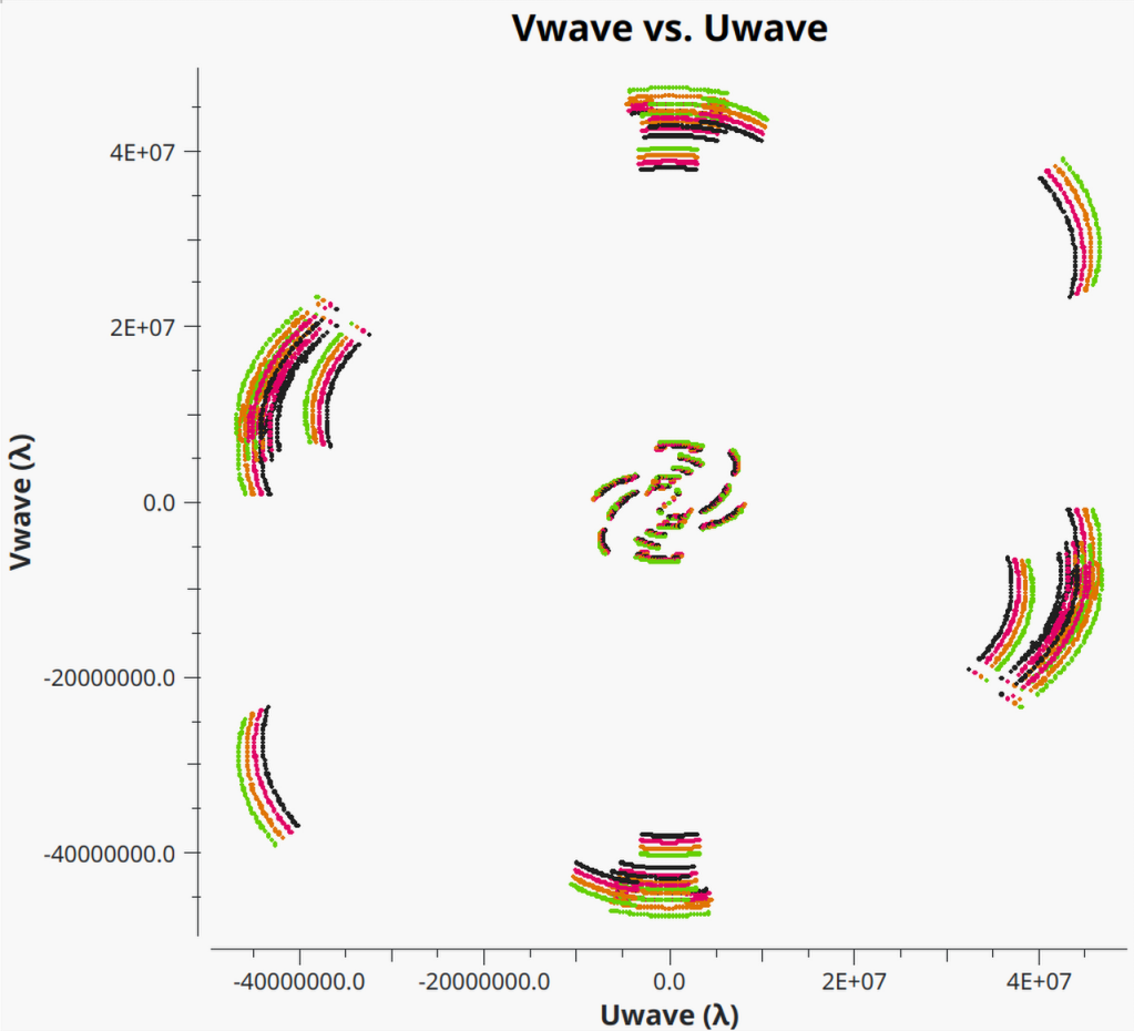
- First let's have a look at the uv-coverage for both sources, using
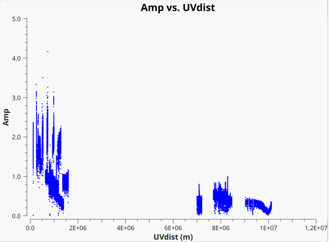
plotms()plotms( vis="3C395_calibrated.ms/", xaxis="uwave", yaxis="vwave", coloraxis="spw" ) - Then let us check the visibility amplitudes vs. uv-distance, with 10s-time averaging
plotms( vis="3C395_calibrated.ms/", xaxis="uvdist", yaxis="amp", avgtime="10", correlation="rr,ll" ) - And finally the visibility phase vs. uv-distance
plotms(
	vis="3C395_calibrated.ms/",
	xaxis="uvdist",
	yaxis="phase",
	avgtime="10",
	correlation="rr,ll"
	)
3C395 (target)
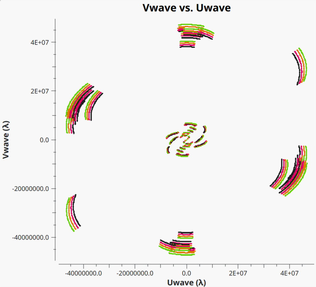
J1848+3219 (phase calibrator)
3C395 (target)
J1848+3219 (phase calibrator)
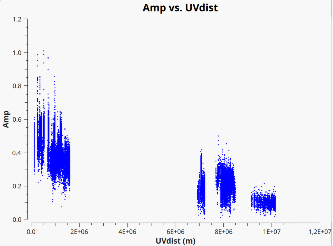
3C395 (target)
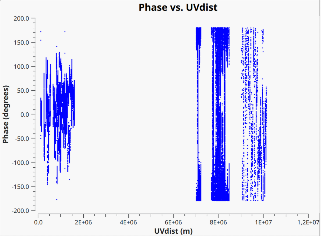
J1848+3219 (phase calibrator)
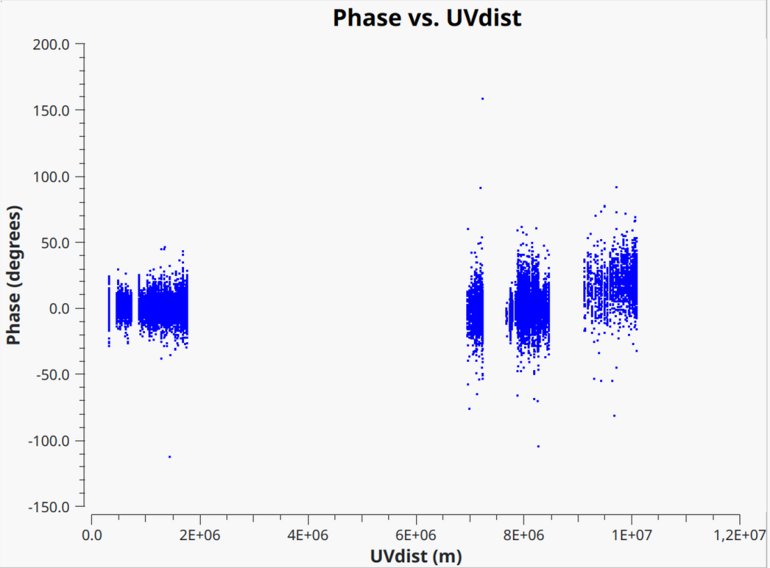
You can clearly see that the scatter in phase and amplitudes is still quite high, which we will try to improve through self-calibration in the following steps.
Note: For typical VLBI data, you will likely have to go through some additional flagging. We have already taken care of flagging the data provided here, so you can skip the flagging process.
2. Imaging the phase calibrator
Before we can perform any kind of self-calibration, we first need to obtain an initial image. For this VLBI observation, we will start with imaging the phase calibrator, which we will later also use to derive the self-calibration solutions and apply them to the target source.
- Let's recall the
tcleantask from the previous tutorials (oricleanfor MacOS), to create a first image of the phase calibrator.Linuxtclean( vis="J1848+3219_calibrated.ms/", imagename="J1848+3219_first_image", specmode="mfs", niter=1500, cycleniter=300, threshold=0, imsize=[512,512], cell="0.3mas", weighting="natural", deconvolver="hogbom", savemodel="modelcolumn", interactive=True )MacOSiclean( vis="J1848+3219_calibrated.ms/", imagename="J1848+3219_first_image", specmode="mfs", niter=1500, cycleniter=300, threshold=0, imsize=[512,512], cell="0.3mas", weighting="natural", deconvolver="hogbom", savemodel="modelcolumn" ) ft(vis="J1848+3219_calibrated.ms/", model="J1848+3219_first_image.model", usescratch=True ) Let's start with a first clean mask similar to this
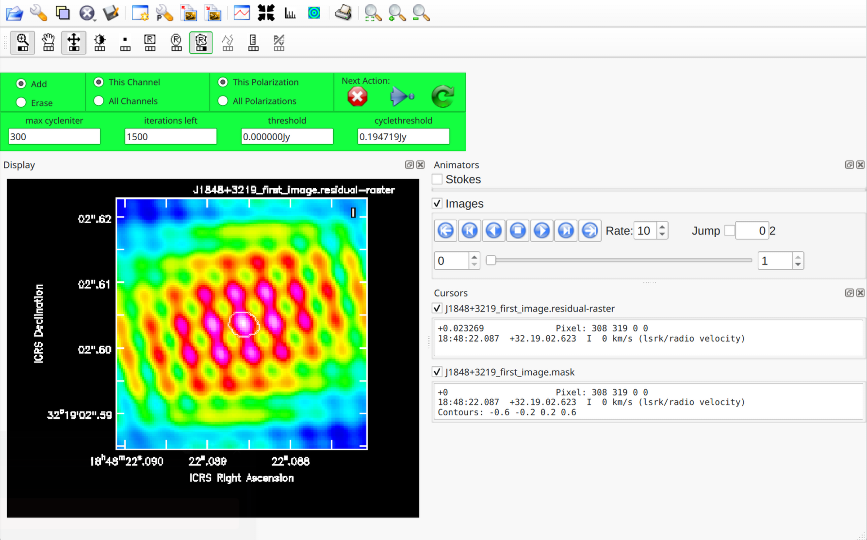
Keep cleaning and adjusting the mask (if required) until your residual map looks similar to this (the bright spots are likely artifacts, so it is best not to put clean windows there):
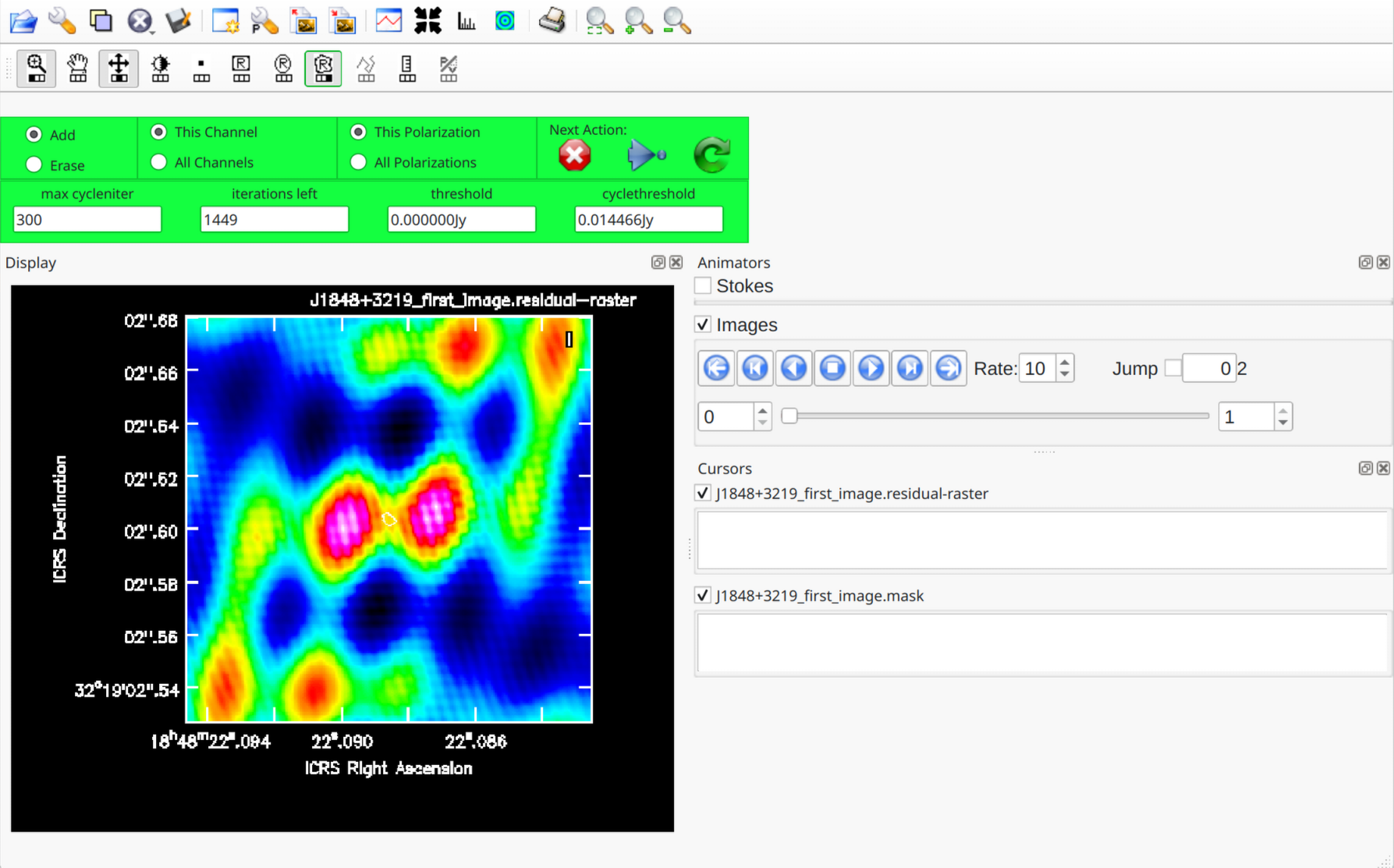
- Now you can close the
tcleanwindow by clicking on the large X. It may take some time as CASA is loading your model into the measurement set. Once this process has finished it is a good idea to check that the CLEAN model that was created describes the data reasonably well. Unfortunately, there is no built-in CASA plot function to do this, but we have created a short plotting script that you may run on your measurement set to compare its model and data visibilities.execfile("compare_model_data.py")The output should look something like this and the CLEAN model should describe the data reasonably well.
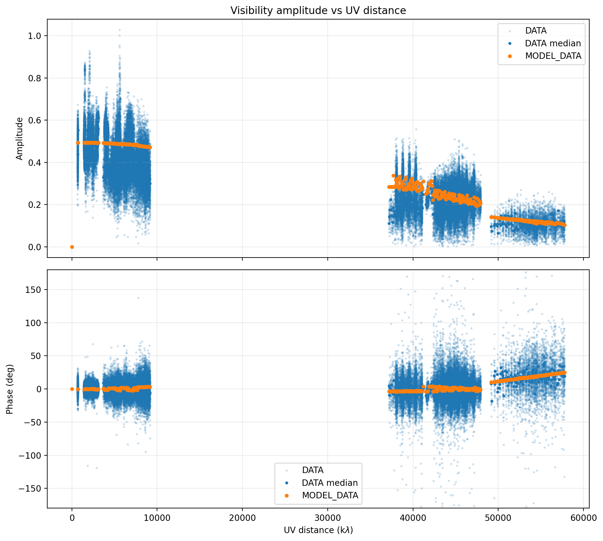
3. Self-calibrate the phase calibrator
Once you are satisfied with your initial CLEAN image of the phase calibrator and the model visibilities describe the data as good as possible, we can start with deriving self-calibration solutions.
-
First, we will start with a phase self-calibration and use a long solution interval
gaincal( vis="J1848+3219_calibrated.ms/", calmode="p", #use "p" to calibrate phases only or "ap" for amplitude and phase caltable="J1848+3219-sc-p1", field="J1848+3219", solint="10min", refant="EF", minblperant=3, minsnr=5 ) -
Now that we created a first phase self-calibration table, we can plot it
and look at the suggested corrections
plotms(
	vis="J1848+3219-sc-p1",
	gridcols=2,
	gridrows=3,
	xaxis="time",
	yaxis="phase",
	iteraxis="antenna",
	coloraxis="spw",
	plotrange=[-1,-1,-180,180]
	)
The plot should look similar to the one shown below. Note that the corrections are typically small. Additionally, for some antennas the solution is missing because they have no data or were already flagged. This is fine and you do not have to worry about it.
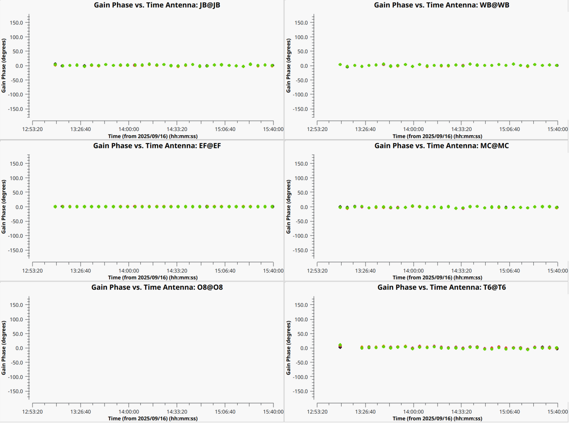
-
Finally, the self-calibration needs to be applied to the measurement set, using the
applycaltaskapplycal( vis="J1848+3219_calibrated.ms/", gaintable=["J1848+3219-sc-p1"], )
4. Iterative self-cal and imaging (hybrid imaging)
After applying the first phase self-calibration, you should go back to step 2
and create a new image of the phase calibrator (ideally, use a different imagename
value for tclean, otherwise you will run into an error).
Once this is done, you can perform self calibration in phase again, but with a shortened solution interval
(2min, as you do not expect faster changes due to the atmosphere).
After another imaging round, if the solutions (in plots) seem to converge to just small improvements,
one can run the self-calibration in amplitude and phase (using calmode="ap" in
gaincal).
For amplitude self-calibration, you do not expect fast changes, but only on the order of ~30 min or more for this dataset.
Therefore, a longer solution interval of half an hour or one hour is sufficient. Below, we provide a short summary of these steps
-
Image the phase calibrator again
Linuxtclean( vis="J1848+3219_calibrated.ms/", imagename="J1848+3219_second_image", specmode="mfs", niter=1500, cycleniter=300, threshold=0, imsize=[512,512], cell="0.3mas", weighting="natural", deconvolver="hogbom", savemodel="modelcolumn", interactive=True )MacOSiclean( vis="J1848+3219_calibrated.ms/", imagename="J1848+3219_second_image", specmode="mfs", niter=1500, cycleniter=300, threshold=0, imsize=[512,512], cell="0.3mas", weighting="natural", deconvolver="hogbom", savemodel="modelcolumn" ) ft(vis="J1848+3219_calibrated.ms/", model="J1848+3219_second_image.model", usescratch=True ) -
Compare model with data
execfile("compare_model_data.py") -
Generate phase calibration table with shorter solution interval of 2 minutes.
gaincal( vis="J1848+3219_calibrated.ms/", calmode="p", #use "p" to calibrate phases only or "ap" for amplitude and phase caltable="J1848+3219-sc-p2", field="J1848+3219", solint="2min", gaintable="J1848+3219-sc-p1", interp=["linear"], refant="EF", minblperant=3, minsnr=5 ) -
Apply both phase calibration tables to the data
applycal( vis="J1848+3219_calibrated.ms/", gaintable=["J1848+3219-sc-p1","J1848+3219-sc-p2"], ) -
Image the phase calibrator again
Linuxtclean( vis="J1848+3219_calibrated.ms/", imagename="J1848+3219_third_image", specmode="mfs", niter=1500, cycleniter=300, threshold=0, imsize=[512,512], cell="0.3mas", weighting="natural", deconvolver="hogbom", savemodel="modelcolumn", interactive=True )MacOSiclean( vis="J1848+3219_calibrated.ms/", imagename="J1848+3219_third_image", specmode="mfs", niter=1500, cycleniter=300, threshold=0, imsize=[512,512], cell="0.3mas", weighting="natural", deconvolver="hogbom", savemodel="modelcolumn" ) ft(vis="J1848+3219_calibrated.ms/", model="J1848+3219_third_image.model", usescratch=True ) -
Compare model with data
execfile("compare_model_data.py") -
Generate calibration table for amplitude and phase calibration.
gaincal( vis="J1848+3219_calibrated.ms/", calmode="ap", #use "p" to calibrate phases only or "ap" for amplitude and phase caltable="J1848+3219-sc-ap", field="J1848+3219", solint="30min", gaintable=["J1848+3219-sc-p1","J1848+3219-sc-p2"], interp=["linear","linear"], refant="EF", minblperant=3, minsnr=5 ) -
Apply all self-calibration tables to the data
applycal( vis="J1848+3219_calibrated.ms/", gaintable=["J1848+3219-sc-p1","J1848+3219-sc-p2","J1848+3219-sc-ap"], ) -
Finally, you can image the phase calibrator one last time, to obtain a final image
Linux
tclean( vis="J1848+3219_calibrated.ms/", imagename="J1848+3219_final_image", specmode="mfs", niter=1500, cycleniter=300, threshold=0, imsize=[512,512], cell="0.3mas", weighting="natural", deconvolver="hogbom", savemodel="modelcolumn", interactive=True )MacOSiclean( vis="J1848+3219_calibrated.ms/", imagename="J1848+3219_final_image", specmode="mfs", niter=1500, cycleniter=300, threshold=0, imsize=[512,512], cell="0.3mas", weighting="natural", deconvolver="hogbom", savemodel="modelcolumn" ) ft(vis="J1848+3219_calibrated.ms/", model="J1848+3219_final_image.model", usescratch=True ) -
You can inspect your final image with
imviewand it will likely look similar to this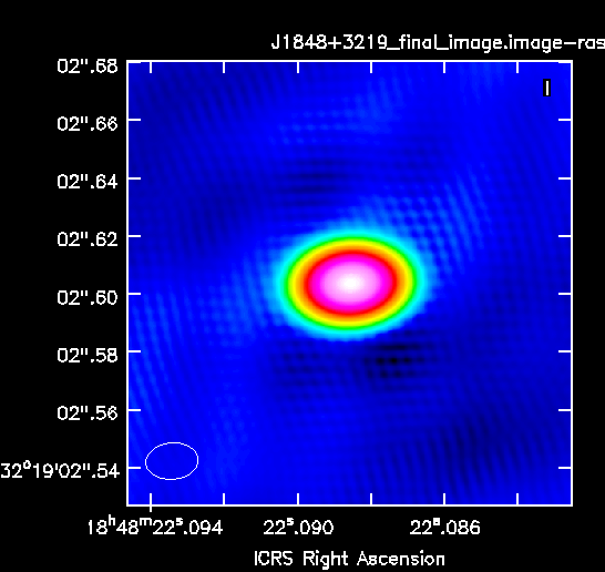
5. Apply solutions to target and image
After finalizing the self-calibration of the phase calibrator, we can easily apply the same solutions to the science target (3C395), and image it.
- Apply amplitude and phase calibration to science target
applycal( vis="3C395_calibrated.ms/", gaintable=["J1848+3219-sc-p1","J1848+3219-sc-p2","J1848+3219-sc-ap"], interp=["linear","linear","linear"] ) -
Image science target
Linux
tclean( vis="3C395_calibrated.ms/", imagename="3C395_final_image", specmode="mfs", niter=1500, cycleniter=300, threshold=0, imsize=[1024,1024], cell="0.3mas", weighting="natural", deconvolver="hogbom", savemodel="modelcolumn", interactive=True )MacOSiclean( vis="3C395_calibrated.ms/", imagename="3C395_final_image", specmode="mfs", niter=1500, cycleniter=300, threshold=0, imsize=[1024,1024], cell="0.3mas", weighting="natural", deconvolver="hogbom", savemodel="modelcolumn" ) ft(vis="3C395_calibrated.ms/", model="3C395_final_image.model", usescratch=True ) -
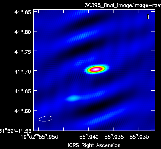
And again, you can plot the final image of the science target with
imview